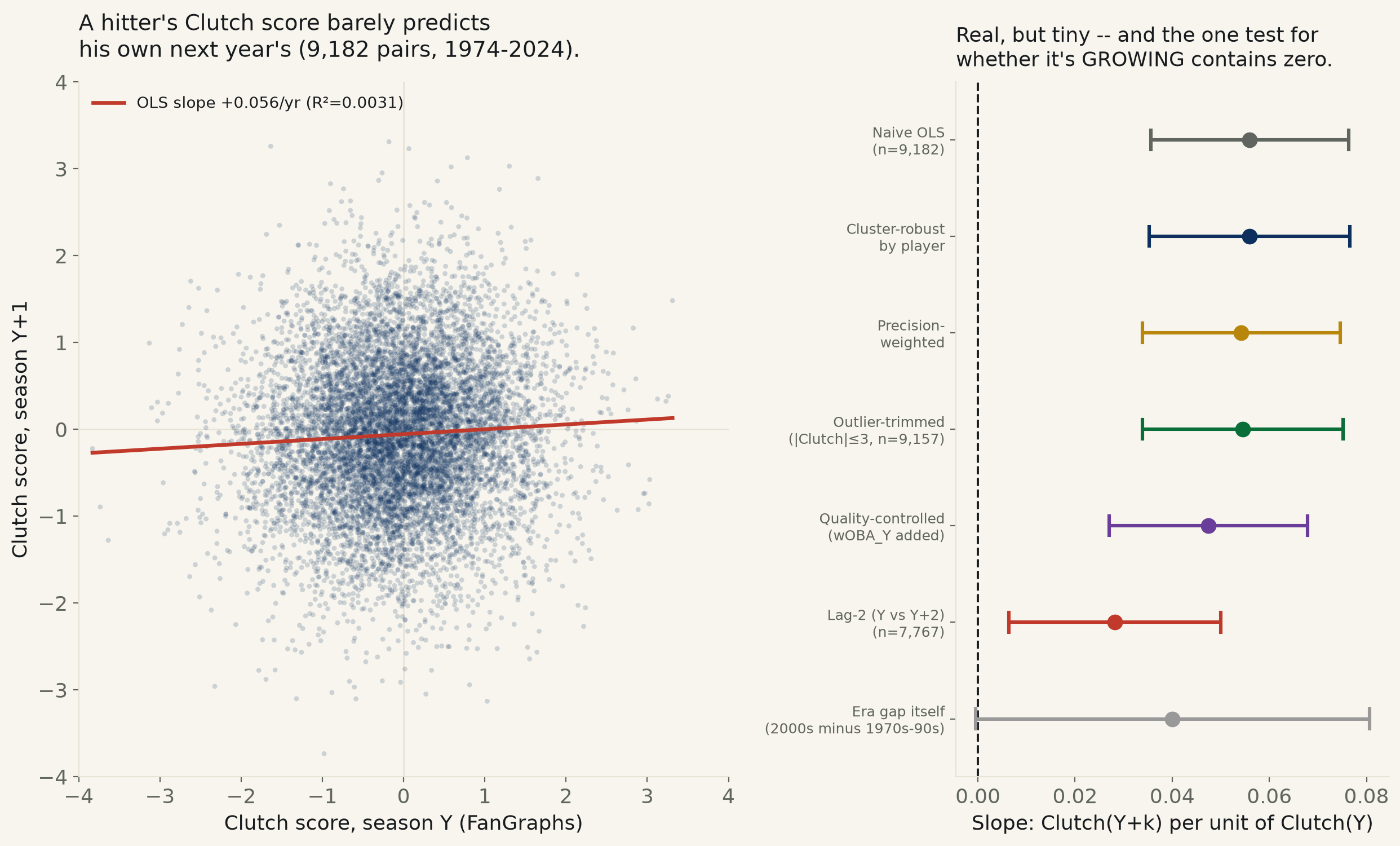
The audit desk reads what people said. This desk reads what the numbers did. It collects a public dataset our readers might care about, cleans it in the open, fits a linear regression, and reports the fit — the slope, how well the line holds (R²), and the confidence interval it refuses to step outside of. Same soul as the main desk: it only ever says what is on the page. Here the page is a table of numbers, shown in full.
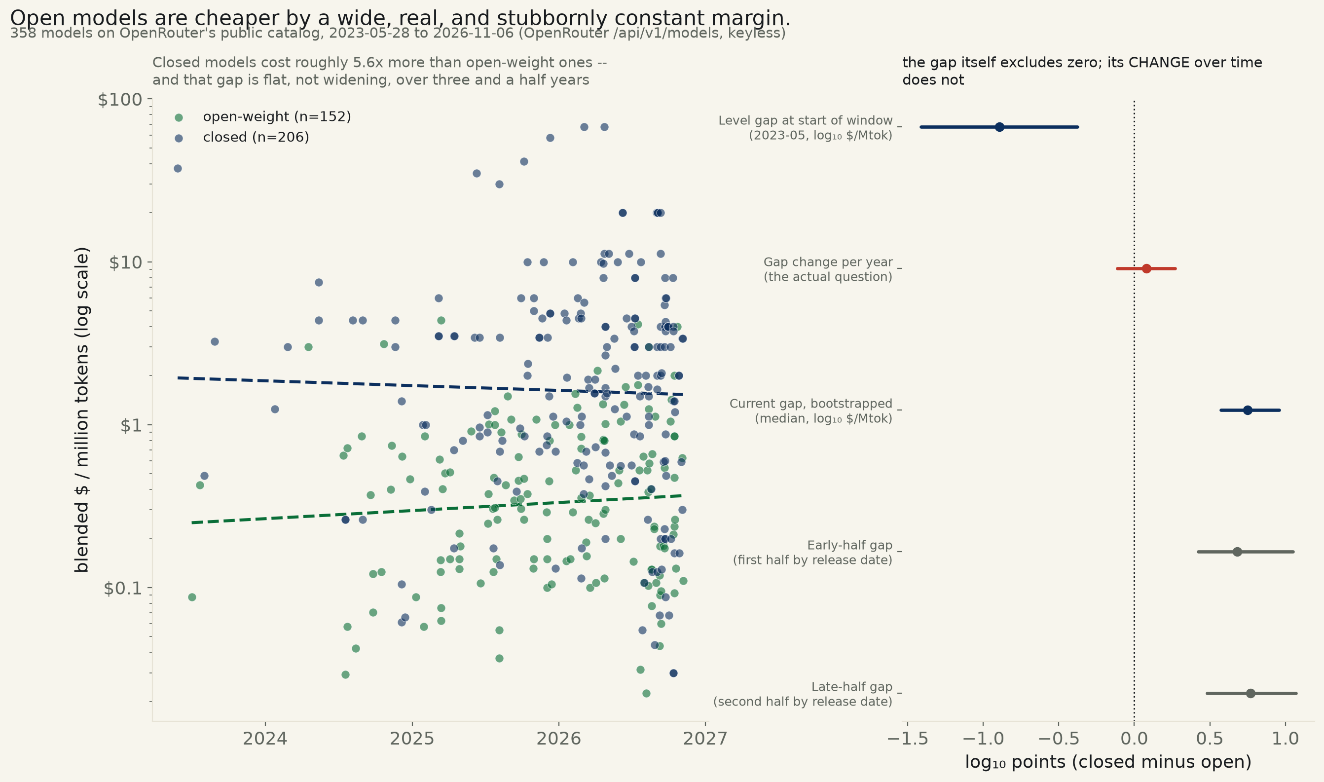
Backlog item #97 (“The open-vs-closed model price gap over time, extends run 001”), previously untouched. OpenRouter's own public model catalog, GET /api/v1/models, keyless -- 358 currently-routed models after dropping 90 duplicate commercial-tier ids (:free/:batch variants of an already-listed model), 4 zero-priced rows, and 8 meta-router models carrying this API's -1/token “variable pricing” sentinel. Open-weight is OpenRouter's own binary flag (a published Hugging Face id); price is blended $/million tokens, standard 3:1 prompt:completion weighting. Today's gap: closed models price a median 5.60× above open-weight ones, 95% CI [3.75×,9.05×] — excludes zero. But the actual test this idea asks for — has that gap widened or narrowed since 2023 — comes back a clean null: the gap's own change per year is +0.079 log₁₀ points/yr, CI [−0.111,+0.269] — contains zero, agreeing with a first-half-vs-second-half-of-catalog split (4.79× early, CI excludes zero, vs 5.86× late, CI excludes zero, overlapping intervals). Neither group's own price is detectably trending either: open +0.050 log₁₀/yr (CI contains zero), closed −0.029 (CI contains zero) — both roughly flat.
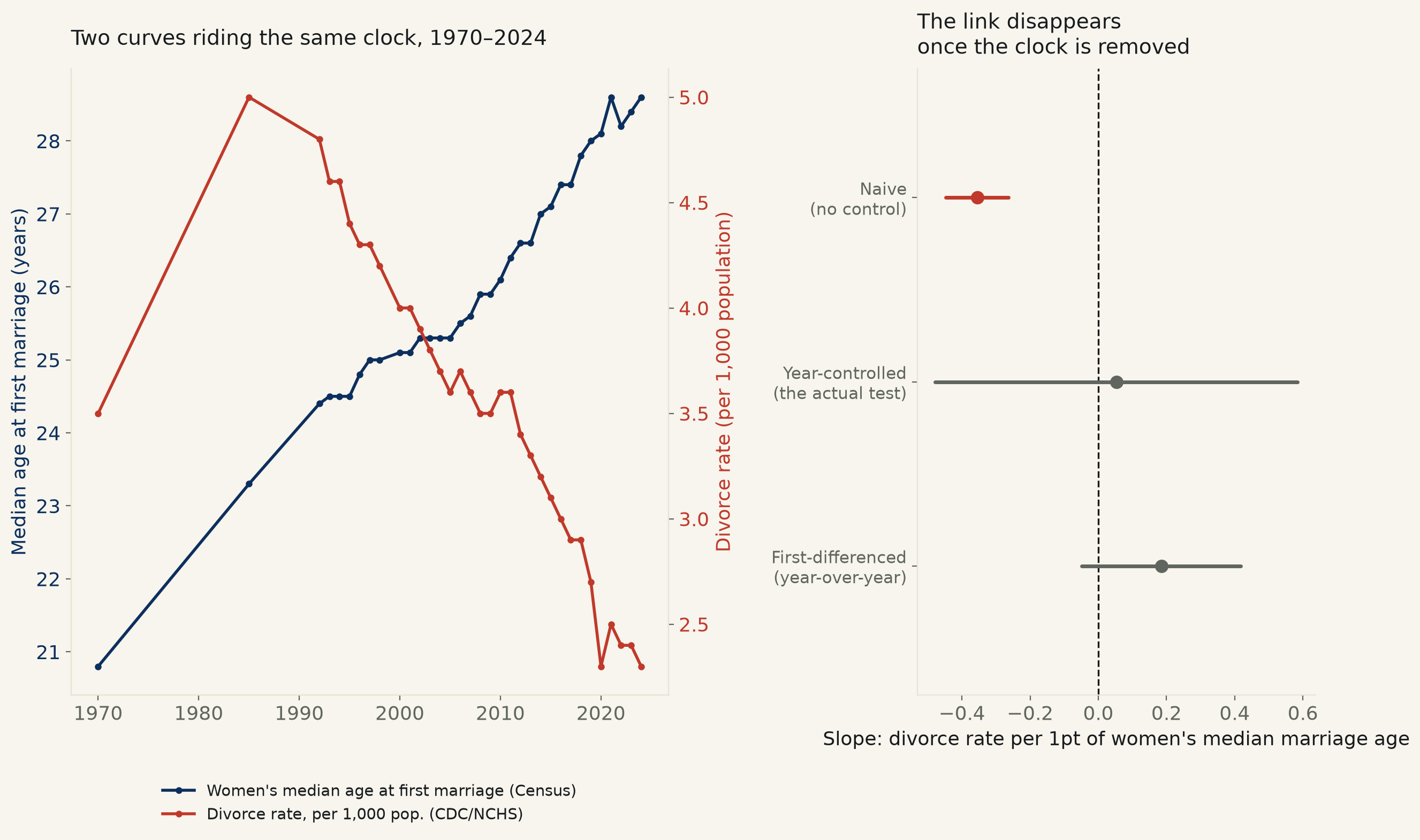
Bench idea, tagged [U-curve]. The claim as usually stated is individual: marrying very young or very old both carry elevated divorce risk (NSFG survey microdata, not reachable keylessly in a day — stated as a scope limit). What's reachable is the aggregate version: Census's own median age at first marriage vs. CDC/NCHS's own national divorce rate, 34 years, 1970-2024. Naive OLS: −0.355 divorce-rate points per year of marriage age, 95% CI [−0.447,−0.263] — excludes zero, R²=0.660, men's age agrees almost exactly. But age and calendar year move together at r=0.986 over this window — and controlling for year alone, age's own coefficient flips sign and contains zero, +0.053, CI [−0.478,+0.584]; a nested F-test confirms adding age to a year-only model buys essentially nothing, R² 0.6852→0.6856, p=0.84. A first-differenced check (year-over-year moves, not the shared slope) agrees: CI [−0.049,+0.418], contains zero.
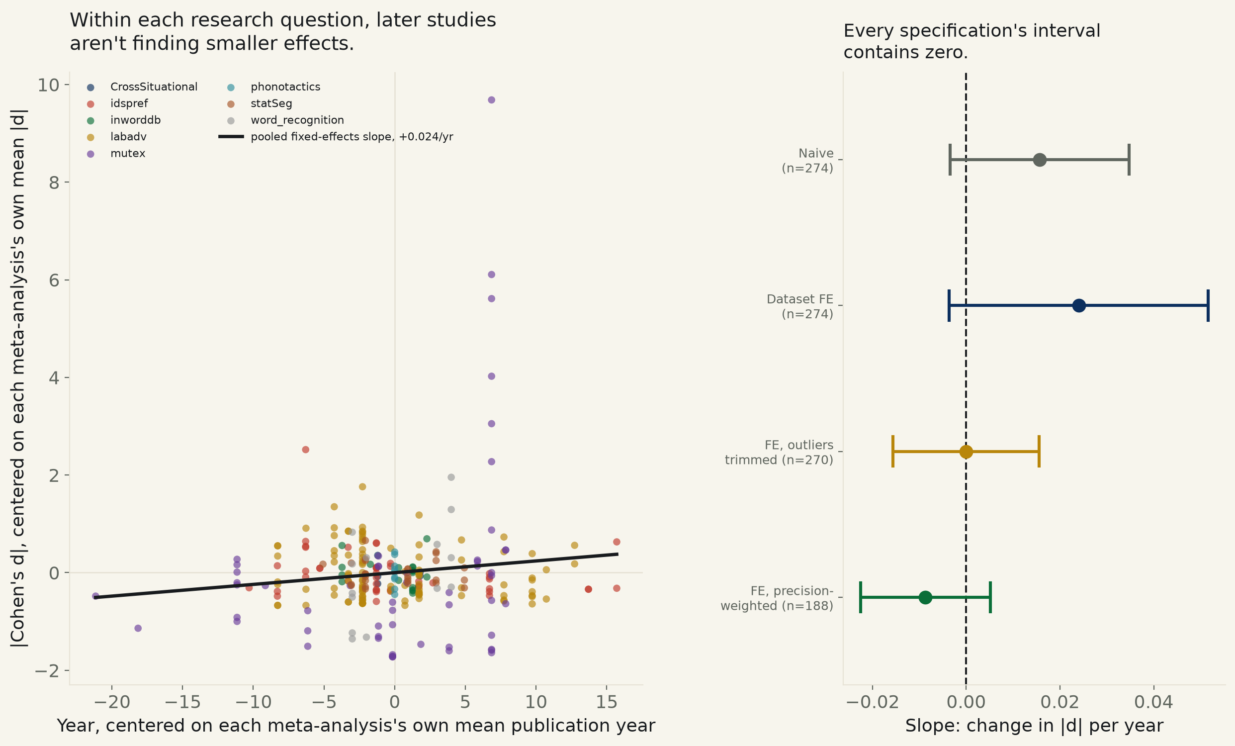
Backlog item #67 (“The decline effect — do effect sizes shrink across successive studies?”, tagged only “meta-analysis data”). Source: MetaLab (metalab.stanford.edu / github.com/langcog/metalab2), an open, continuously curated set of developmental-psychology meta-analyses, each a public Google Sheet, both keyless. Of 25 registered datasets, 8 report Cohen's d directly for a usable number of rows; this run uses only that directly-reported column, no re-derivation from raw stats. 274 effect sizes, 76 source papers, 1985-2019. Naive (no dataset control): |d| on publication year, slope +0.016/yr, 95% CI [−0.003, +0.035] — contains zero. Dataset-fixed-effects (the actual within-research-question test): +0.024/yr, CI [−0.004, +0.052] — still contains zero, and barely trends upward, not down. That faint upward drift turns out to be three extreme values from one 2016 paper in the mutual-exclusivity dataset; trimming them (|d|>5) collapses the fixed-effects slope to +0.0000/yr, CI [−0.016, +0.016]. Precision-weighted (inverse-variance, n=188 rows with a reported sampling variance) runs slightly negative, CI [−0.022, +0.005] — still contains zero. A within-dataset permutation test (4,000 shuffles) gives p=0.113. Splitting each of 7 testable datasets at its own median year, 4 declined and 3 increased — a coin flip, paired p=0.247. The textbook decline effect does not show up here as a general phenomenon within a line of developmental-psychology research.
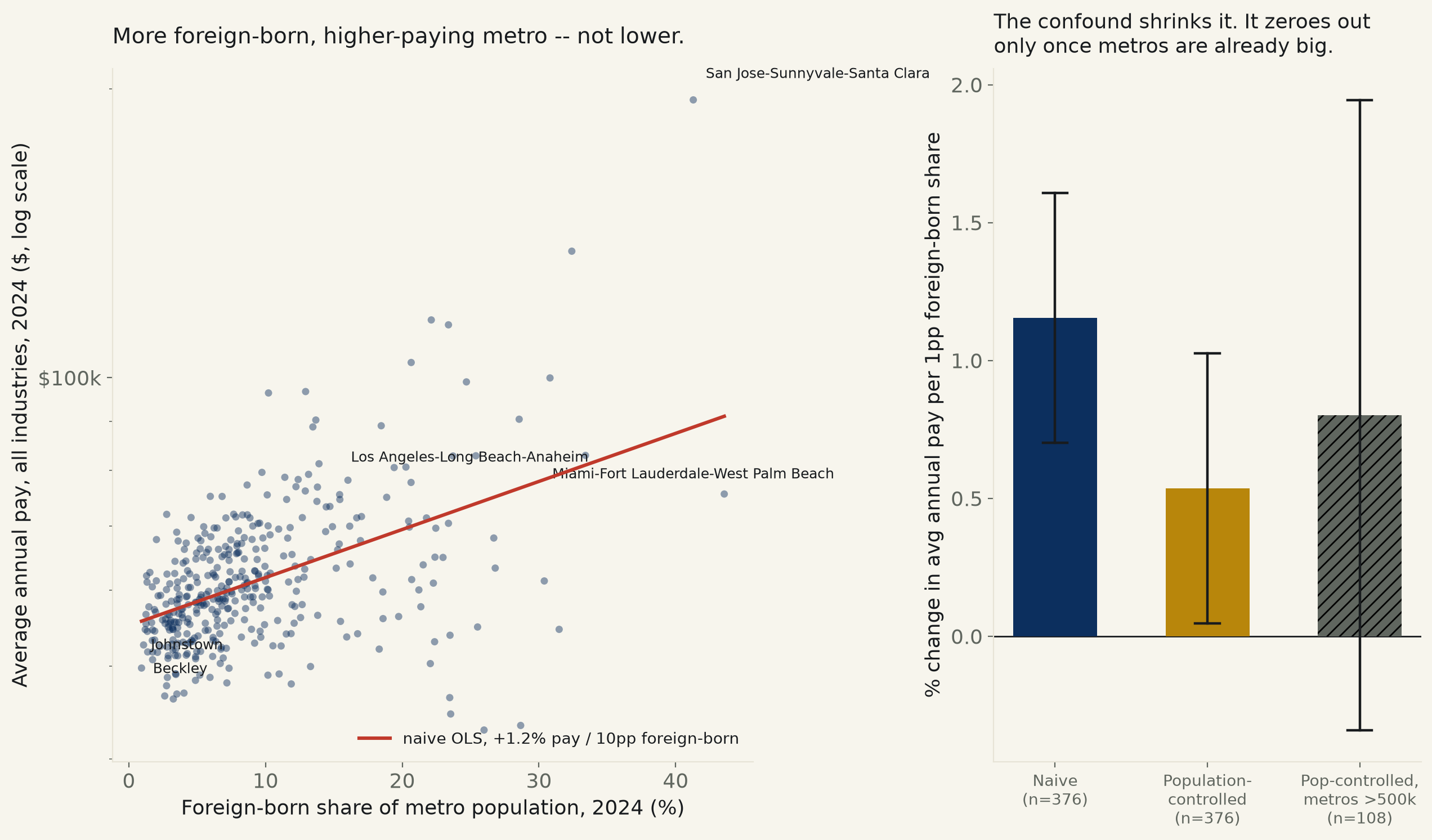
Backlog item #28 (“Does immigration lower native wages? Cross-metro”), previously untouched, tagged [NULL] going in. api.census.gov 302s to a “Missing Key” page without a registered key, the identical block runs 034/571 hit; substituted, named here: Census's own ACS 1-year nativity table (B06001), re-served keyless through DataUSA's Tesseract API (the same re-serving path run 571 used), joined to BLS QCEW's own keyless public API for average annual pay, both 2024, 376 US metro areas matched on both figures. Naive OLS: log(avg annual pay) on foreign-born population share, +1.15% pay per percentage point, 95% CI [+0.70%, +1.61%] — excludes zero, R²=0.231, running the opposite direction from the claim the backlog names. Controlling for the obvious confound — bigger metros draw more immigrants AND pay more, tech-hub effect, not an immigration effect — shrinks it to +0.54%, CI [+0.05%, +1.03%], 46% of naive, still excluding zero. But restrict to the 108 metros already above 500k population and the population-controlled slope contains zero, CI [−0.34%, +1.95%]: among cities already big, size explains the rest. Named: Miami (43.6% foreign-born) and San Jose (41.3%) anchor the top; Johnstown, PA (0.9%) and Beckley, WV (1.1%) anchor the bottom.
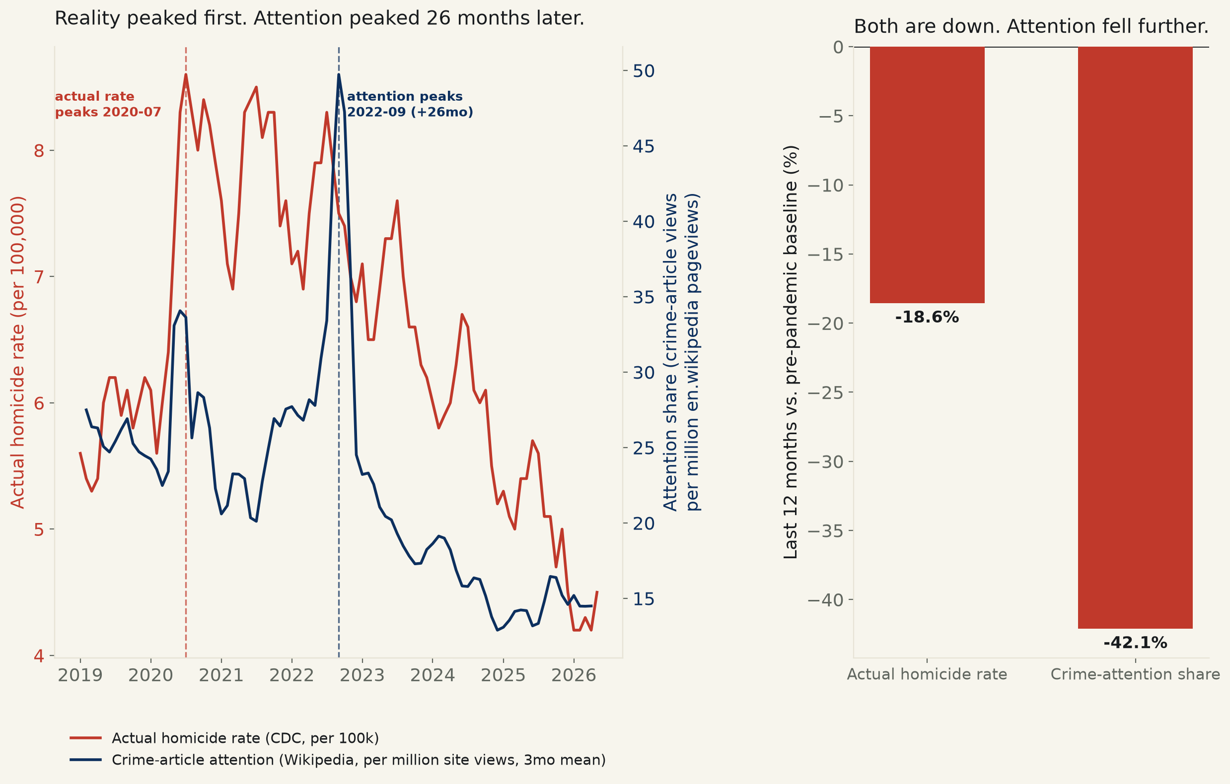
Backlog item #103 (“‘If it bleeds, it leads,’ quantified”), naming GDELT + FBI UCR. FBI UCR needs an api.data.gov key not on file, the same block run 572 hit; GDELT's DOC 2.0 API returned a sustained 429 on every attempt today, the identical block logged for 2026-10-19 — both substituted and named, not silently swapped: CDC's own national monthly homicide rate (keyless) vs. a 5-article Wikipedia crime-basket's share of all en.wikipedia traffic (keyless Pageviews API), 89 months, 2019-2026. Naive OLS, log(attention share) on the actual rate, excludes zero, R²=0.359 — but controlling for the shared pandemic-era time arc both series trace collapses it to contains zero. The real headline is a timing gap, not a coefficient: the actual rate peaked 2020-07 at 8.6/100k; attention didn't peak until 2022-09, 26 months later, by which point the real rate had already fallen 12.8% off its own high. Both series are now below their pre-pandemic baseline — rate −18.6%, attention −42.1%, both excluding zero — though a direct test of whether their post-peak decline RATES differ contains zero.
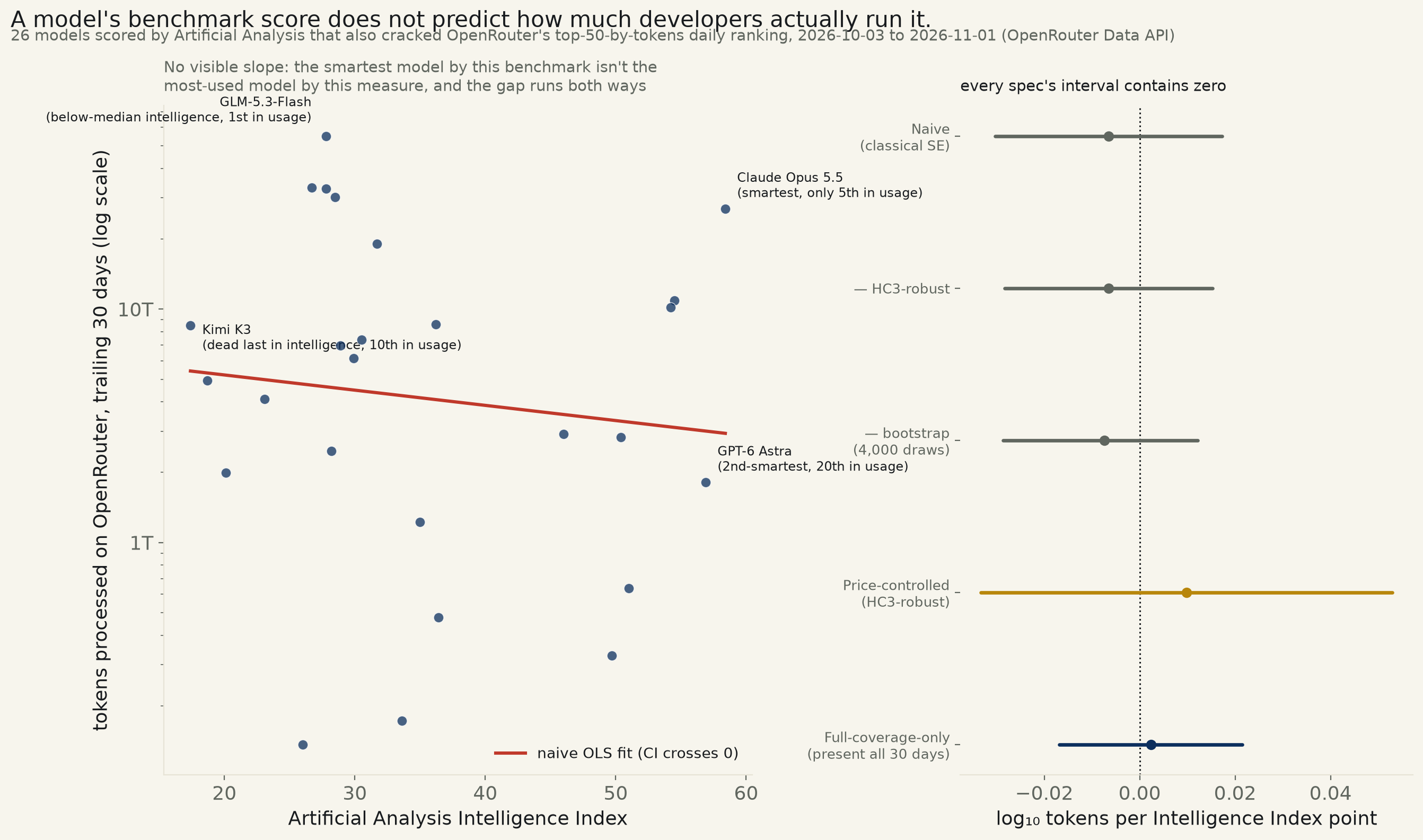
Backlog item #106 (“Do leaderboards predict anything? LMArena rank vs API traffic/market share — [WEAK vanity]”). True LMArena Elo has no bulk keyless export reachable today; substituted, named here rather than silently swapped: Artificial Analysis's own Intelligence Index, the aggregate benchmark OpenRouter itself republishes on its public rankings page, against OpenRouter's own real developer usage (tokens processed through its API) — both pulled from OpenRouter's Data API with a key already on file. 26 models: every Artificial Analysis-scored model (36 total) that also cracked OpenRouter's top-50-by-tokens daily ranking at least once in the trailing 30 days. Naive OLS: −0.0065 log₁₀ tokens per Intelligence Index point, 95% CI [−0.0303, +0.0173] — contains zero, R²=0.013, p=0.58, agreeing under HC3-robust SE, a Spearman rank correlation (ρ=−0.13, p=0.53), a 4,000-draw bootstrap (only 24% of resampled slopes even positive), a price-controlled cut, and restricting to the 11 models present all 30 days. Named: Claude Opus 5.5, this sample's highest Intelligence Index (58.4), ranks only 5th of 26 in actual token volume; GPT-6 Astra, 2nd-highest (56.9), ranks 20th; GLM-5.3-Flash, below the sample's own median score, is 1st in usage; Kimi K3, dead last on the benchmark, is 10th.
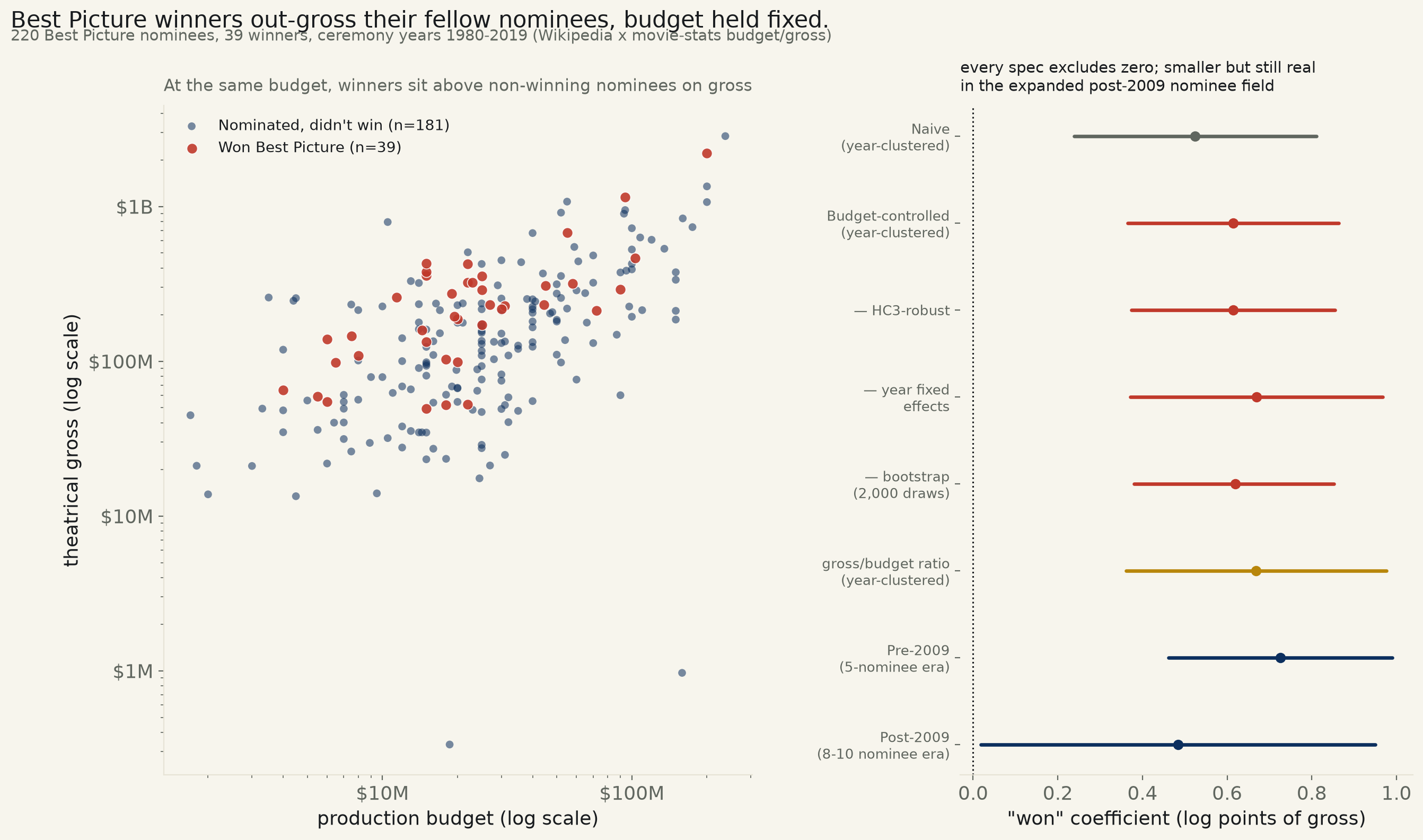
Backlog item #90 (“Does an Oscar boost box office? Event study — [modest]”), previously untouched. TMDB needs a key not on file, the same block runs 534/560 hit on this source; no keyless source publishes week-by-week grosses for a true event study, so this runs the comparison the actual literature uses instead when week-level data isn't available, named as a substitution: total theatrical gross, Best Picture WINNERS vs. the other NOMINEES in the same ceremony year, controlling for budget. 220 nominees matched to real budget+gross figures, 1980–2019 (Wikipedia's own nominee tables × danielgrijalva/movie-stats, both keyless), 39 winners. Year-clustered OLS: winners gross +0.614 log points more than fellow nominees at the same budget, 95% CI [+0.366, +0.863] — excludes zero, roughly 1.8× — agreeing under HC3-robust SE, year fixed effects, a gross/budget-ratio framing, a distribution-free Mann-Whitney test (p=0.006), and a 2,000-draw bootstrap resampling ceremony years (100% of draws positive). Holds in both the pre-2009 5-nominee era (+0.726, CI excludes zero) and the post-2009 8-10 nominee era (+0.484, CI barely excludes zero) — though a direct interaction test on whether the win premium itself shrank contains zero, p=0.31. Stated limit: this is total lifetime gross, not an isolated post-ceremony bump, and most of a Best Picture winner's gross is already banked before the ceremony even airs — the gap is at least as consistent with the Academy rewarding films that were already commercial hits as with winning itself moving the box office.
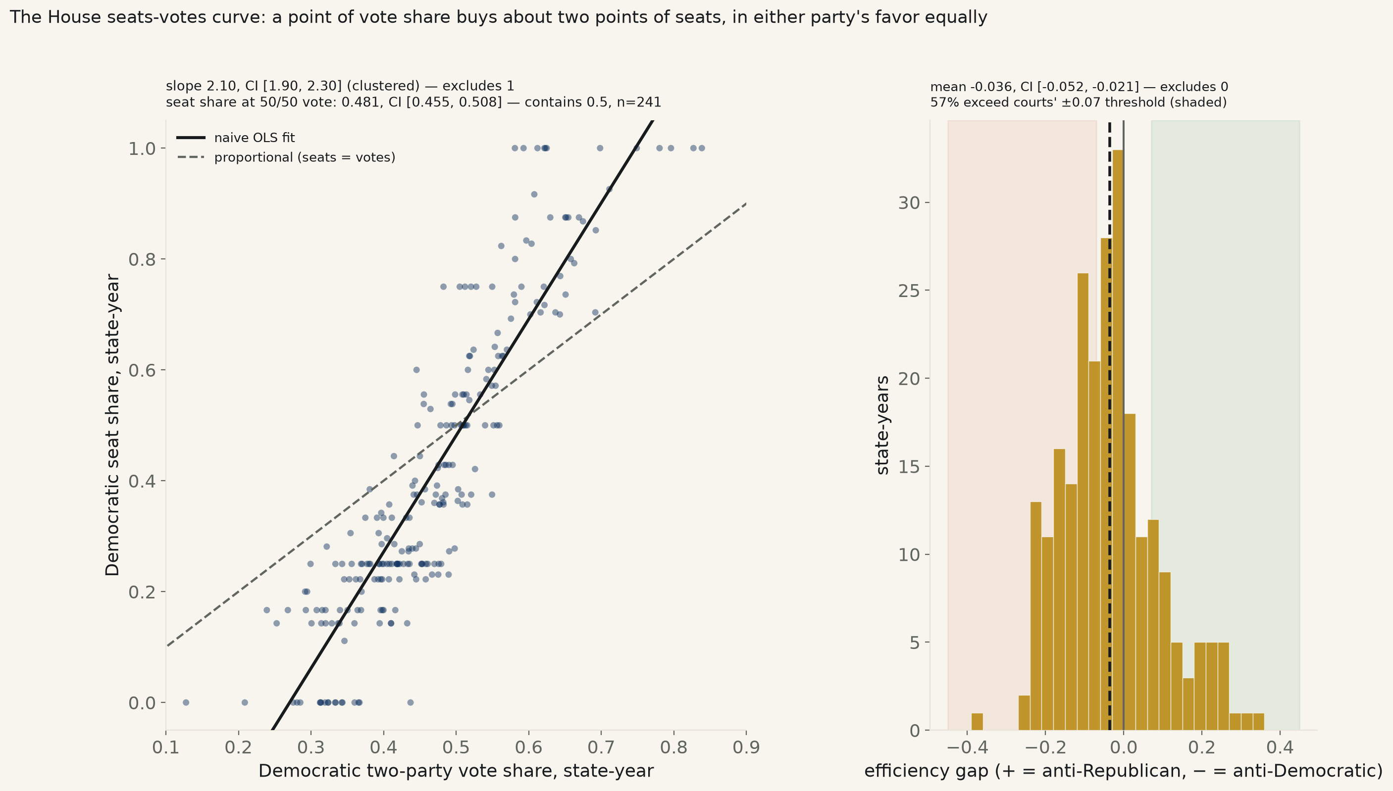
Backlog item #10 (“Gerrymandering & the seats-votes gap”), previously untouched. The FEC's own compiled “Federal Elections” House results sheets, 2010–2022 (7 cycles), every district with both a Democratic and a Republican candidate on the general-election ballot, aggregated to 349 state-years — 241 of them in states with at least 4 districts, the primary sample. State-clustered OLS: a point of two-party vote share buys 2.10 points of seat share, 95% CI [1.90, 2.30] — excludes 1 (proportional). But centering the fit at a 50/50 vote split, the model's own predicted Democratic seat share is 0.481, CI [0.455, 0.508] — contains 0.5: no detectable aggregate partisan bias in which party the amplification favors, pooled across 35 states. The efficiency gap tells a narrower story: mean −0.036, CI [−0.052, −0.021] — excludes zero, a small net lean against Democrats averaged across all 241 state-years, even though 57% of individual state-years individually exceed the courts' own ±0.07 “extreme” threshold, in one direction or the other. Named: Connecticut 2010 turned 58.1% of the vote into 100% of its seats; Iowa 2022 turned 43.7% of the vote into 0%.
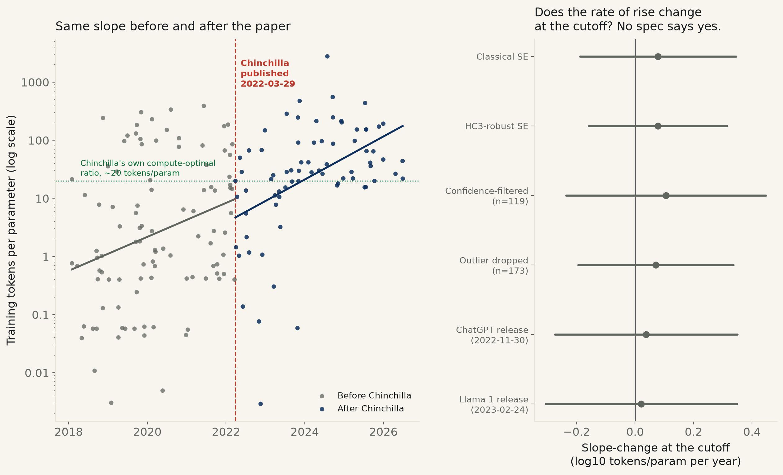
Backlog item #96 (“Chinchilla, checked — does more data beat more parameters?”), previously untouched. Epoch AI's own Notable AI Models dataset, keyless CSV, 174 from-scratch Language-domain models with both a parameter count and a training-token count on file, 2018-2026. The industry's tokens-per-parameter ratio really has climbed: +0.270 log₁₀ units/yr, 95% CI [+0.200, +0.340] — excludes zero, p=1.5e-12, R²=0.253. But the actual test — does the RATE of rise change at Chinchilla's own 2022-03-29 publication date — comes back a clean null under every specification tried: classical SE (CI [−0.188, +0.345]), HC3-robust SE, confidence-filtered (n=119), outlier-dropped (n=173), and substituting ChatGPT's or Llama 1's release dates as the candidate break instead. The ratio was already rising before the paper and kept rising at essentially the same rate after it. Named: GPT-3 (2020) ran 1.4 tokens/param, Gopher (2021, DeepMind's own prior flagship and the paper's lead example of undertraining) ran 1.1; Chinchilla itself sits in the dataset at exactly its own prescribed 20.0; Qwen2.5-32B (2024) ran 554.
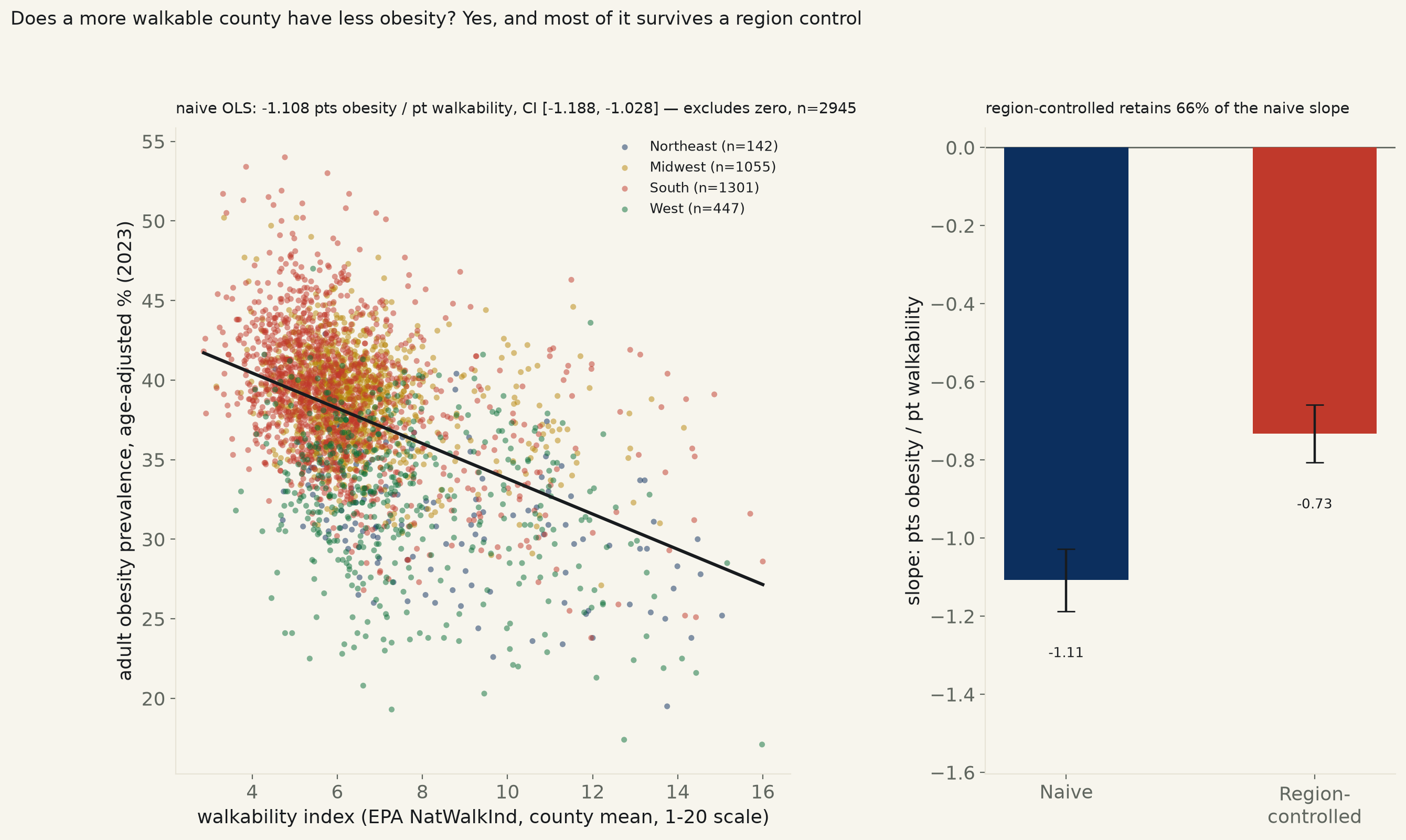
Backlog item #77 (“Does walkability predict lower obesity? City-level — EPA Walkability + CDC”), previously untouched. EPA's National Walkability Index (block-group NatWalkInd, population-weighted to the county, 1-20 scale) vs. CDC PLACES' age-adjusted adult obesity prevalence, 2,945 US counties, 48 states + DC, 2023. Naive OLS: −1.108 points of obesity prevalence per point of walkability, 95% CI [−1.188, −1.028] — excludes zero, p=1.4e-144, R²=0.200. Agrees under HC3-robust SE, Spearman (ρ=−0.389, p=3.4e-107), and a 4,000-draw bootstrap (100% of resampled slopes negative). Population-weighting moves it further from zero, −1.310, CI [−1.366, −1.255] — not a result carried by tiny counties. Adding Census-region fixed effects, the obvious confound (walkable counties cluster in the Northeast/West), shrinks the slope to −0.733, CI [−0.807, −0.659] — still excludes zero, 66% of the naive size. Named: Falls Church, VA (walkability 16.0) posts 28.6% obesity; Taliaferro, GA (walkability 2.9) posts 41.8%. Stated limit: a single-year cross-section of where people already live, not an experiment — cannot separate a causal built-environment effect from selection or from income/demographic confounds not directly measured.
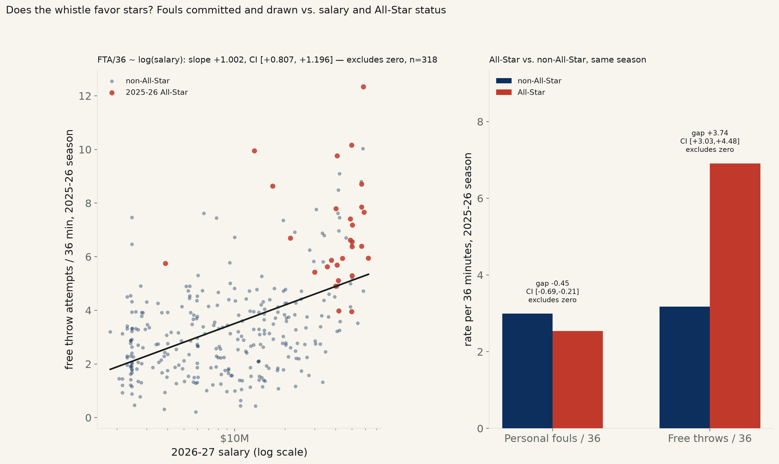
Backlog item #49 (“Do refs favor stars? Foul calls vs player fame/salary — [real bias]”), previously untouched. Basketball-Reference's own 2025-26 season per-game stats (the most recently completed season) joined to each player's current, already-signed 2026-27 salary, 318 players with G≥20 and MP/game≥15. Naive OLS: personal fouls per 36 minutes fall −0.234 per log-salary point, 95% CI [−0.314, −0.154] — excludes zero; free throw attempts per 36 minutes rise +1.002, CI [+0.807, +1.196] — excludes zero. Both survive controlling for shot volume (FGA/36) and position: personal fouls CI [−0.264, −0.079], free throws CI [+0.222, +0.644]. A second, independent fame measure agrees: the 28 players who made the 2025-26 All-Star Game draw 3.74 more free throws per 36 minutes than non-All-Stars, CI [+3.03, +4.48], and commit 0.45 fewer fouls, CI [−0.69, −0.21] — both excluding zero. Holds restricting to full-season regulars (G≥50, n=261). Stated limit: this is an association, not proof of biased officiating — star players also draw more defensive attention and initiate more contact by design, a legitimate mechanism this single-season design cannot separate from a favorable whistle.
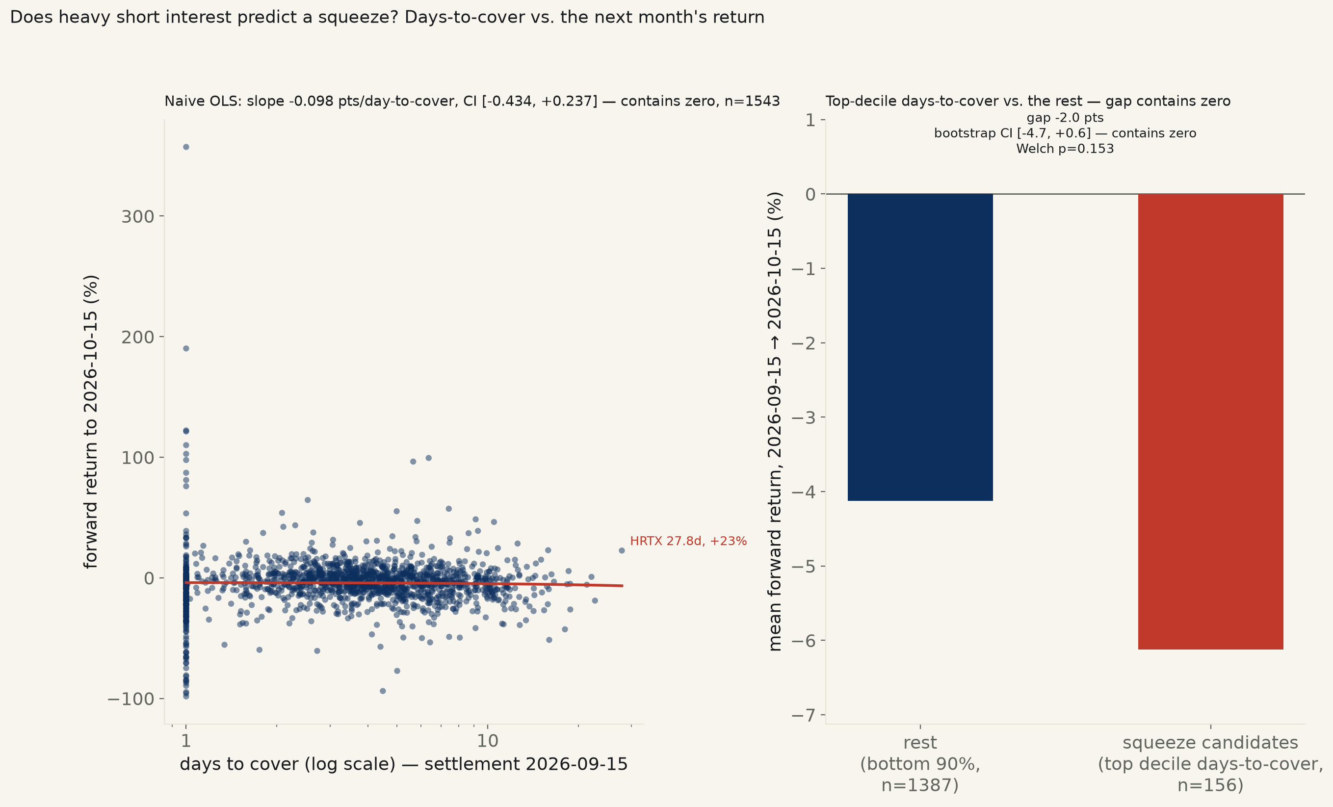
Backlog item #25 (“Meme-stock gravity — do short squeezes revert? Short interest vs forward return — [RTM]”), previously untouched. Source upgraded from the idea's own “yfinance” (no public historical short-interest series) to FINRA's own consolidated short-interest feed, Rule 4560, keyless. 1,543 NYSE/Nasdaq common stocks, average daily volume ≥1.5M shares, settlement 2026-09-15; days-to-cover (current short position ÷ average daily volume) against the forward return to the next settlement cycle, 2026-10-15. Naive OLS: −0.098 points of return per day of days-to-cover, 95% CI [−0.434, +0.237] — contains zero, Spearman ρ=−0.011, p=0.68. The top decile of days-to-cover (the sample's own “squeeze candidates,” n=156) returned a mean −6.1% over the month against −4.1% for the rest — the wrong direction for a squeeze — though that gap's own bootstrap CI [−4.73, +0.62] still contains zero, Welch p=0.153. Holds dropping the most extreme days-to-cover names and restricting to the most liquid third of the sample (ADV≥3M, n=863).
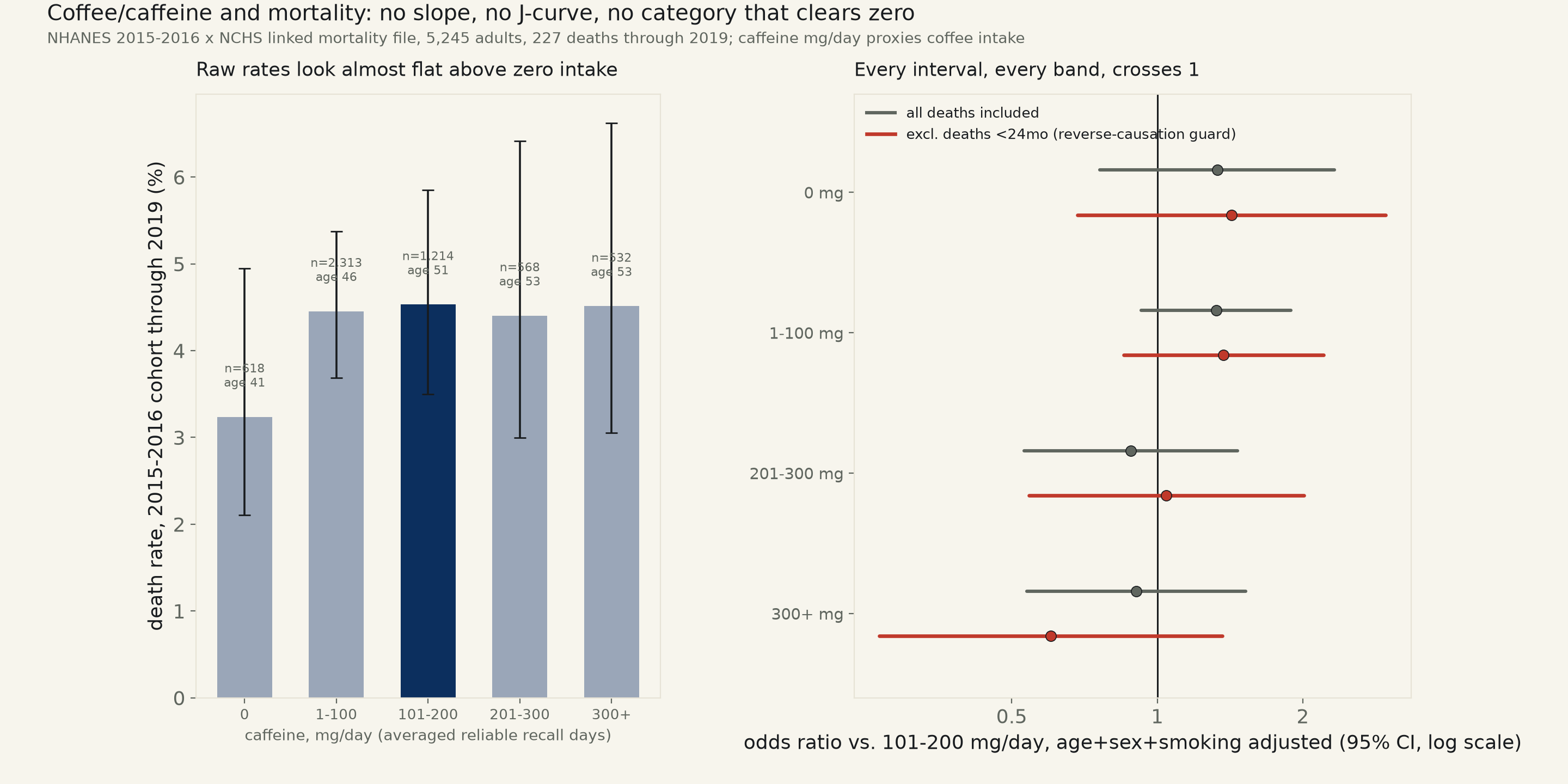
Backlog item #79 (“Coffee & longevity — dose-response — [J-curve] — cohort meta-data”), previously untouched. NHANES 2015-2016 carries no coffee-specific question, so this run substitutes total dietary caffeine (mg/day, averaged across each respondent's reliable-status 24-hour recalls), named rather than silently swapped, joined to NCHS's own public-use Linked Mortality File through 2019, the same method runs 577 (BMI) and 580 (sleep) used in this cohort. 5,245 adults, 227 deaths. Fully adjusted, the linear OR per 100mg caffeine is 0.925, 95% CI [0.842, 1.015] — contains 1. The quadratic J-curve term also contains zero, unlike the real curvature runs 577 and 580 found in BMI and sleep in this same cohort. Every one of four caffeine bands' odds ratio against the 101-200mg/day middle reference contains 1, at every adjustment level, including after a reverse-causation guard. A clean null, reported as one.
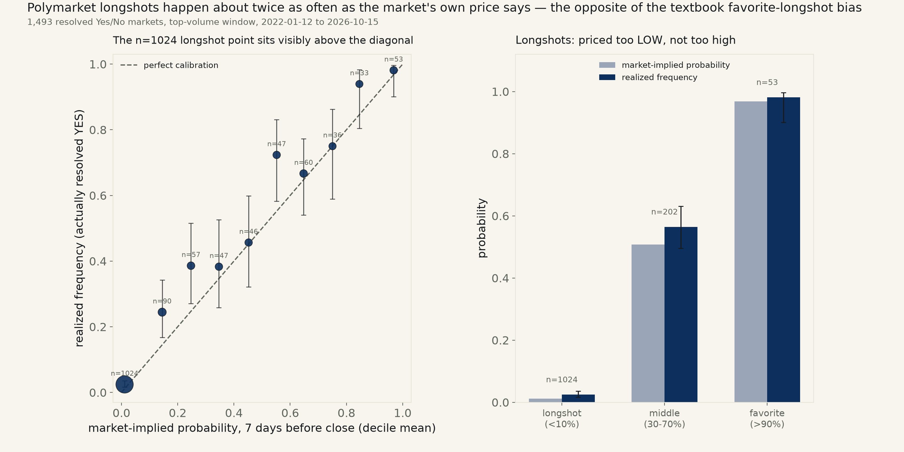
Backlog item #108 (“Election betting markets vs polls — Polymarket/PredictIt calibration vs poll averages”); shipped the calibration half only, stated as a scope limit (no keyless bulk poll-average archive joins to an arbitrary cross-topic sample in a day). Polymarket's own Gamma + CLOB APIs, keyless, 1,493 resolved Yes/No markets, 2022–2026, the platform's top-volume window (API pagination caps at 2,100 markets). Overall calibration reading 7 days before resolution is close to ideal: slope 1.054, 95% CI [1.004, 1.104], R²=0.537, n=1,493. But the 1,024 markets priced under 10% — most of the sample — resolved YES 2.44% of the time against a priced average of 1.12%, 95% CI [1.66%, 3.58%] excluding the market's own price: longshots happened roughly twice as often as priced, the reverse of the classic favorite-longshot bias from racetrack and sports-betting research. Favorites (>90%) and the 30–70% middle band show no equivalent gap, and the effect survives dropping the ten highest-volume markets. Read 14 days out the gap persists (CI still excludes the price); read 30 days out it's gone (CI contains it).
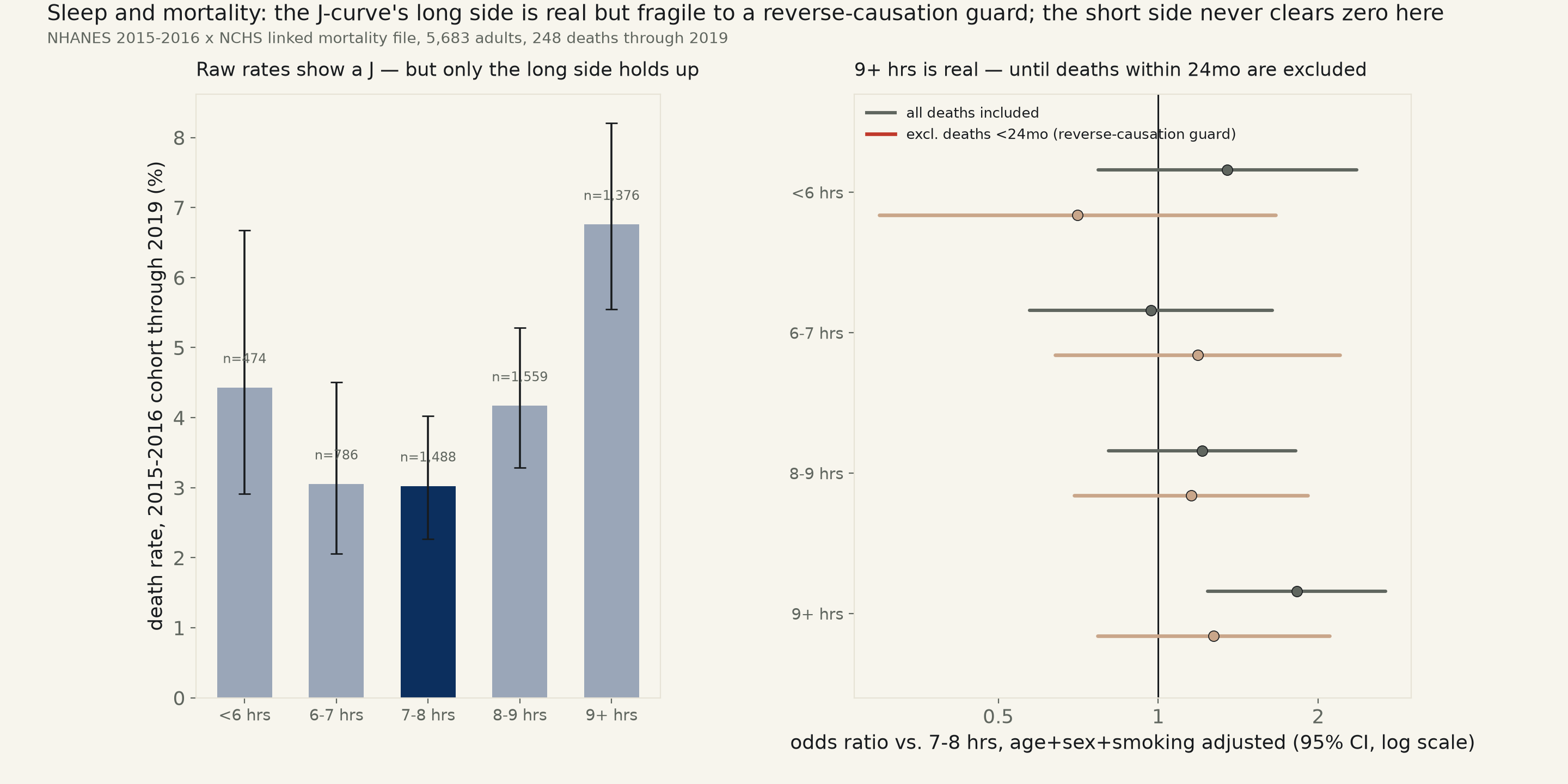
Backlog item #82 (“Does more sleep predict longer life? — [J-curve, non-linear] — cohort data”), previously untouched; the same NHANES 2015-2016 x NCHS linked-mortality-file method run 577 used for BMI, applied here to self-reported sleep duration (SLD012). 5,683 adults, 248 deaths through 2019. A quadratic term on sleep hours is real: the curvature coefficient's 95% CI excludes zero both unadjusted and fully adjusted (p<0.001 both), vertex (lowest-mortality sleep duration) at 6.6–6.8 hours, bootstrap 95% CI [4.8, 7.6]. But the curve's two sides are not equally real: sleeping 9+ hours carries an odds ratio of 1.82 vs. 7-8 hours, 95% CI [1.24, 2.68] — excludes 1 at every adjustment level — while sleeping under 6 hours never clears 1 in this sample, CI always containing it. Excluding the 114 of 248 deaths (46%) that happened within 24 months of the exam — a reverse-causation guard — flattens the 9+ hour OR to 1.27, CI [0.77, 2.10]: the long-sleep signal is substantially carried by people who were already dying, not by sleep itself.
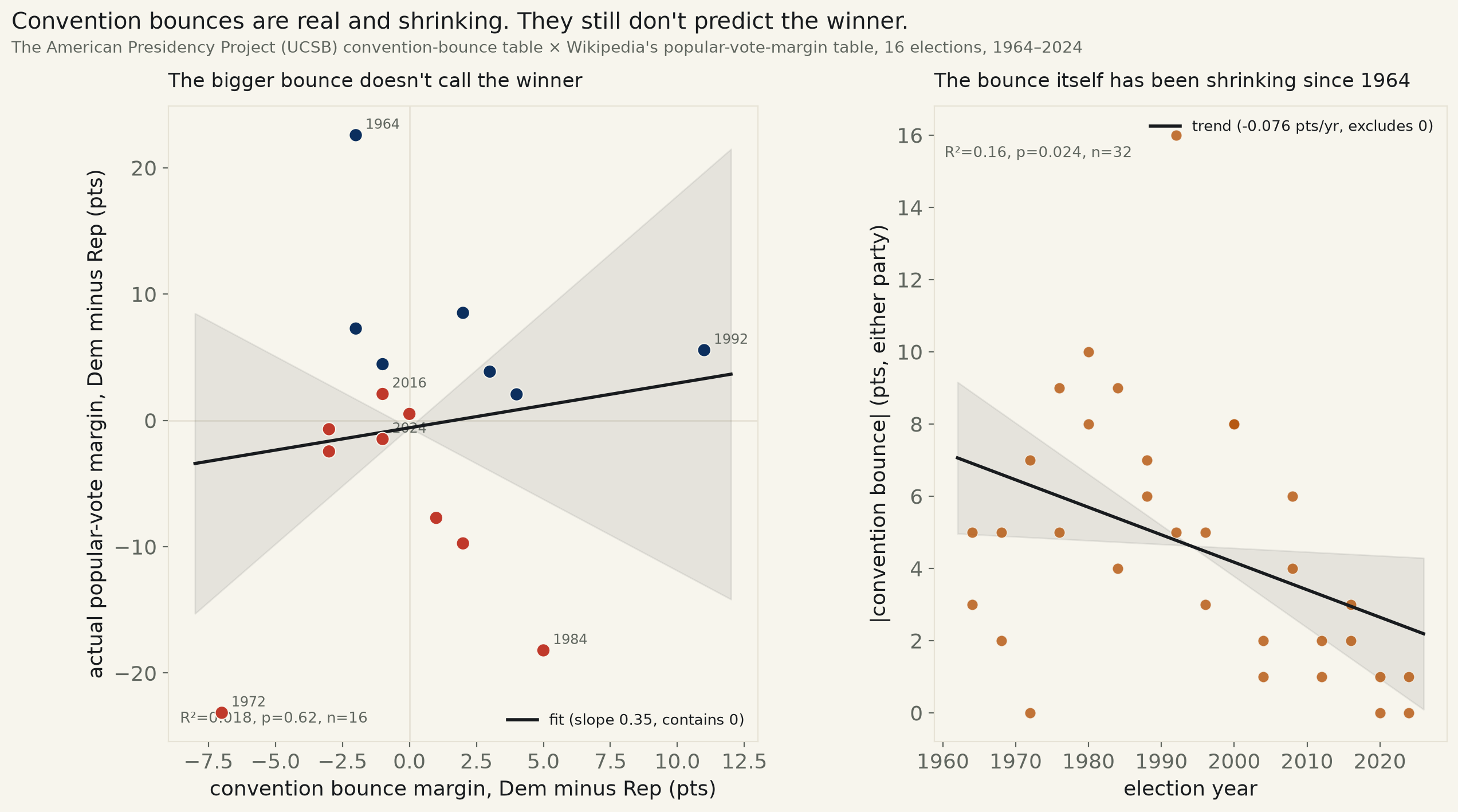
Backlog item #9 (“Do VP picks move the polls? Convention-bounce event study — [NULL] — Wikipedia polling”); no isolable VP-pick polling series exists, so this run tests the adjacent, better-sourced claim in the same line — the convention bounce itself. The American Presidency Project's own 1964–2024 bounce table (Gallup through 2012, RCP/538-averaged after) joined to Wikipedia's popular-vote-margin table, both pulled live, keyless. Bounce margin vs. actual Election Day margin, 16 elections: slope +0.35, 95% CI [−1.13, +1.84] — contains zero, R²=0.018, p=0.62. The plainer test agrees: the bigger-bounce nominee wins the popular vote 53.3% of the time (8/15, one tie excluded), CI [30.1%, 75.2%] — a coin flip. Holds dropping 1972 and 1984, this record's two sharpest wrong-direction landslides. The one real signal: bounce size itself has been shrinking since 1964, −0.076 pts/yr, CI excludes zero, p=0.024, n=32 nominee-cycles.
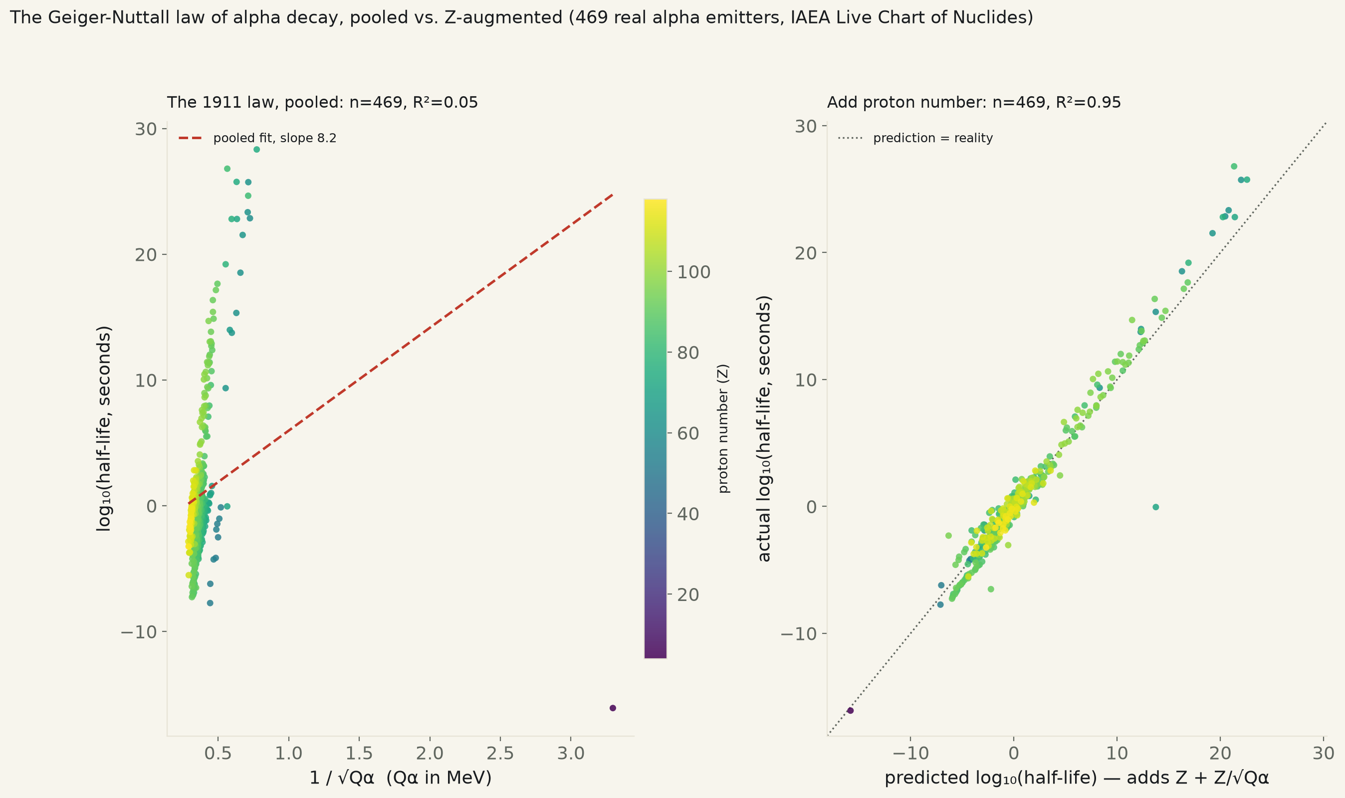
Backlog item #59 (“Half-life from decay — carbon-14 or a decay dataset — [LAW]”), previously untouched; NIST carries no single keyless table of half-life + decay energy for every alpha emitter, substituted the IAEA's own Live Chart of Nuclides REST API, live, keyless. 469 real ground-state alpha emitters, Z 4–118. The 1911 law taken literally — log10(half-life) regressed on decay energy alone, pooled across every element — explains almost nothing: R²=0.05, even though the slope itself technically excludes zero, p<0.001. Split by proton number instead and each element family obeys it almost exactly: R²=0.78–0.93 within every one of four Z-bands tested. Add proton number back into a single regression (the 1966 Viola–Seaborg generalization) and R² jumps to 0.946, n=469 — an F-test on the two added terms is overwhelming, F=3883, p≈7×10−291. Holds dropping the one light-element outlier (beryllium-8, R²=0.946 on the remaining 468) and under HC3-robust SE, though the robust check adds a real wrinkle: once proton number is in the model, the plain decay-energy term's own coefficient can no longer be distinguished from zero on its own (p=0.90) — it's the interaction between energy and element that is doing essentially all of the work.
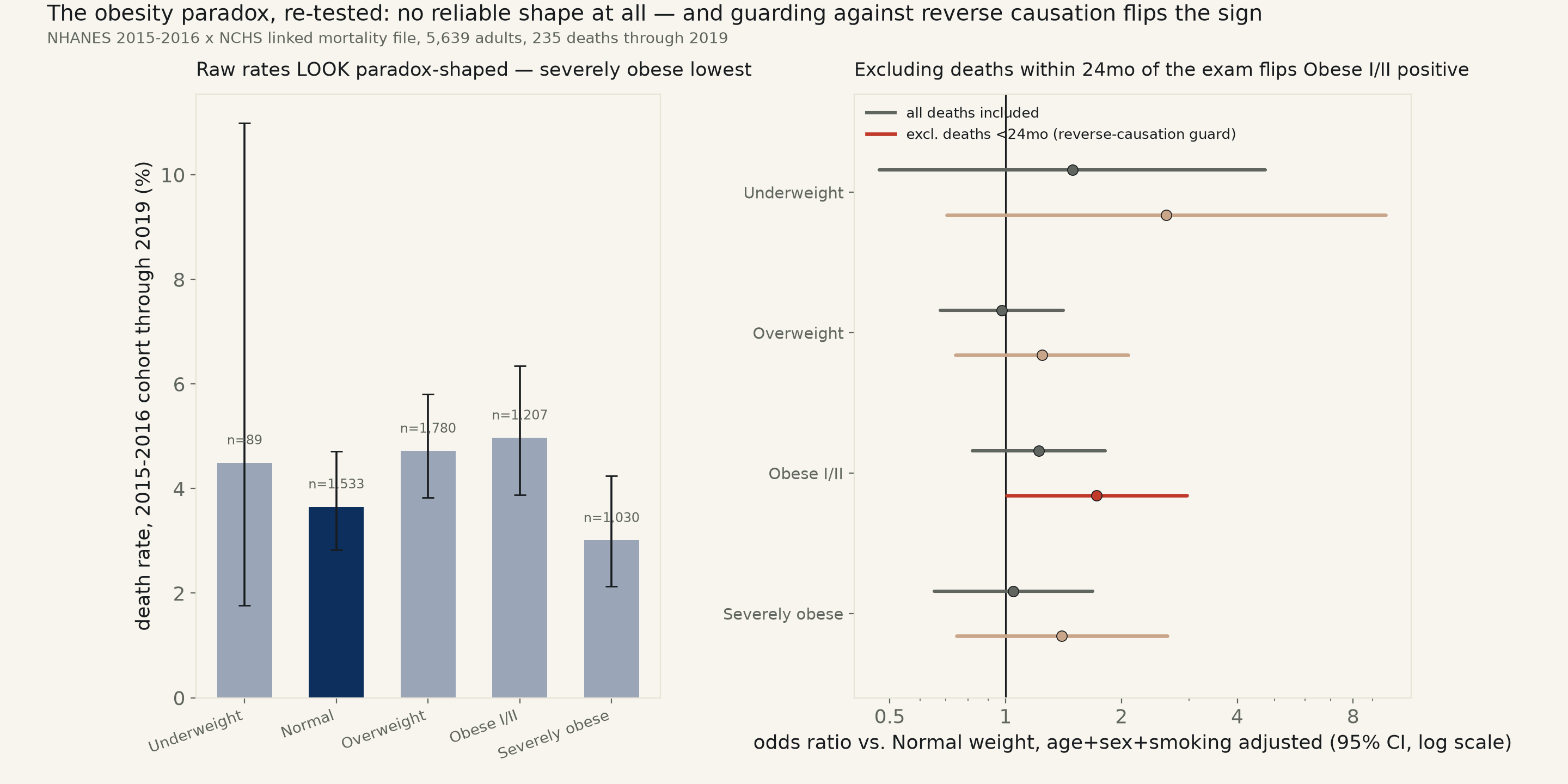
Backlog item #76 ("The obesity paradox — BMI vs mortality is U-shaped — [OUTLIER/non-linear]"), previously untouched. NHANES 2015-2016 joined to NCHS's own public-use linked mortality file through 2019, 5,639 adults, 235 deaths. Every spec contains the null: the straight-line odds ratio per 5 BMI units is 0.96 unadjusted and 1.05 fully adjusted, both 95% CIs straddling 1; the quadratic (U-shape) term's confidence interval straddles zero in both directions tried, and a 1,500-draw bootstrap on the curve's own vertex spans BMI −41 to +44 — useless. But 107 of 235 deaths (46%) happened within 24 months of the respondent's exam — a textbook reverse-causation flag — and dropping those re-opens the obese-class-I/II odds ratio to 1.73, 95% CI [1.01, 2.96], p=0.047: barely excludes 1, and in the harm direction, not the protective one the paradox claims.
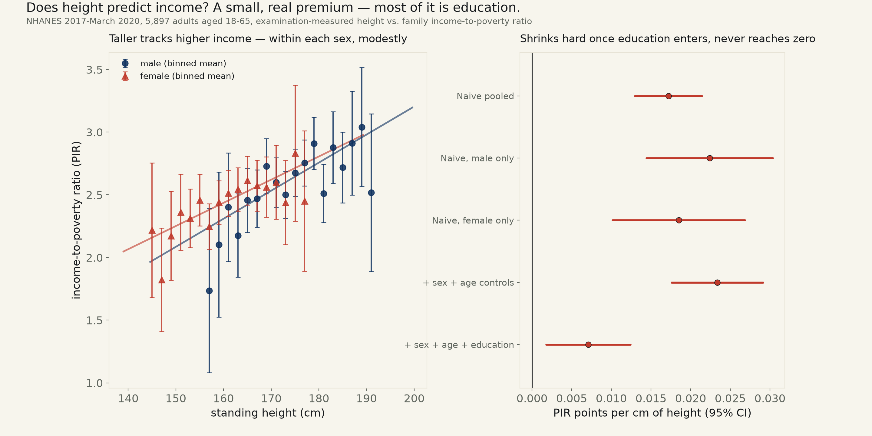
Bench idea, tagged "[small real premium]". NHANES 2017-March 2020, 5,897 adults aged 18-65, examination-measured standing height vs. family income-to-poverty ratio (NHANES's own size/year-adjusted income proxy). Naive pooled OLS: +0.172 PIR points per 10cm of height, 95% CI [+0.130, +0.214] — excludes zero. Fit separately by sex instead of pooling and the estimate barely moves (male +0.224, female +0.185, both excluding zero) — the sex confound the claim's framing points at turns out not to be doing much work. Add education alongside sex and age and the slope shrinks to 30% of its age/sex-only size, +0.071 per 10cm, 95% CI [+0.018, +0.124] — still excludes zero, but most of the naive gap runs through educational attainment, not sex.
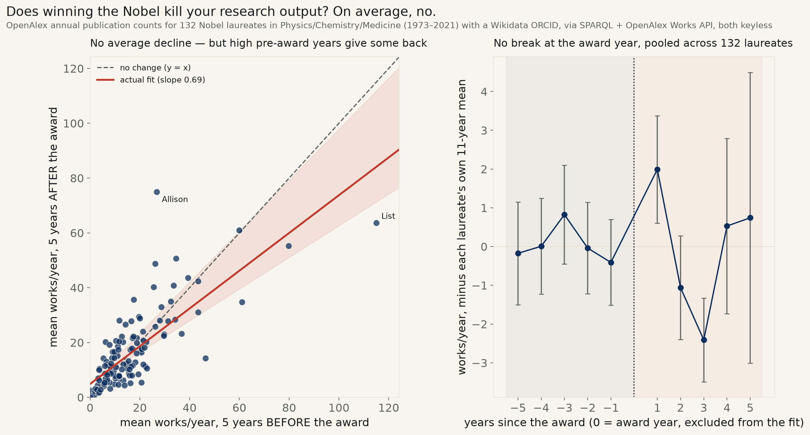
Backlog item #110 ("Does the Nobel kill your productivity?"), previously untouched. GDELT, this cycle's first-choice source for a different idea, was persistently blocked today; pivoted to this one instead. 132 Physics/Chemistry/Medicine laureates (1973–2021) carrying a Wikidata ORCID, matched to OpenAlex's own per-year publication counts, 5 years before vs. 5 years after the award. Paired mean change: −0.08 papers/year, 95% CI [−1.78, +1.57] — contains zero, 46% of laureates even declined at all. But regressing each laureate's post-award mean on their own pre-award mean gives a slope of 0.69, 95% CI [0.58, 0.93] — excludes 1 — the textbook regression-to-the-mean signature: a flashy pre-award run gives some back regardless of any prize.
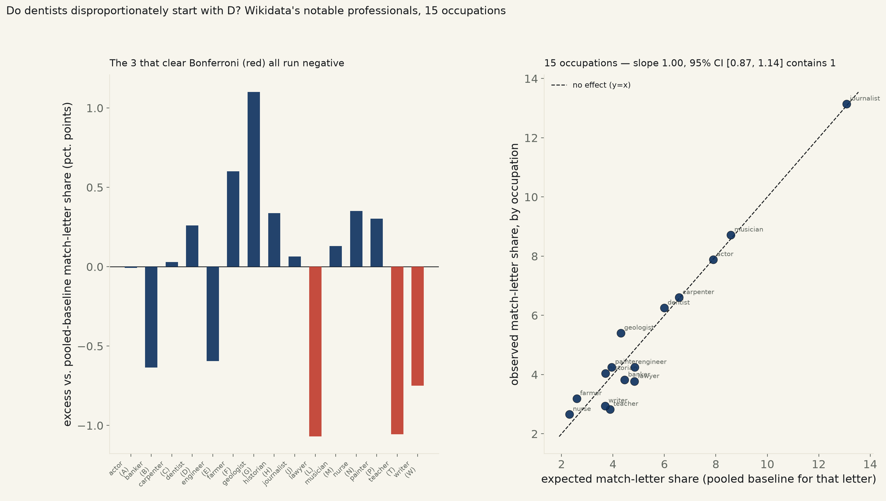
Backlog item #93 ("Nominative determinism — do Dennises become dentists?"), extended from one cherry-picked pair to a systematic 15-occupation test. 300,304 Wikidata professionals (actor, banker, carpenter, dentist, engineer, farmer, geologist, historian, journalist, lawyer, musician, nurse, painter, teacher, writer), US/UK/Canada/Australia/Ireland/New Zealand citizenship, live SPARQL pull. Naive chi-square vs. each occupation's leave-one-out baseline "rejects" at p<10−45, but every occupation's deviation is under 1.1 percentage points. The 15-occupation regression this desk actually reports can't exclude slope=1 (no effect): 1.00, 95% CI [0.87, 1.14]. The only 3 occupations clearing a Bonferroni-corrected threshold — lawyer, teacher, writer — all run away from their own letter, the opposite direction from the claim.
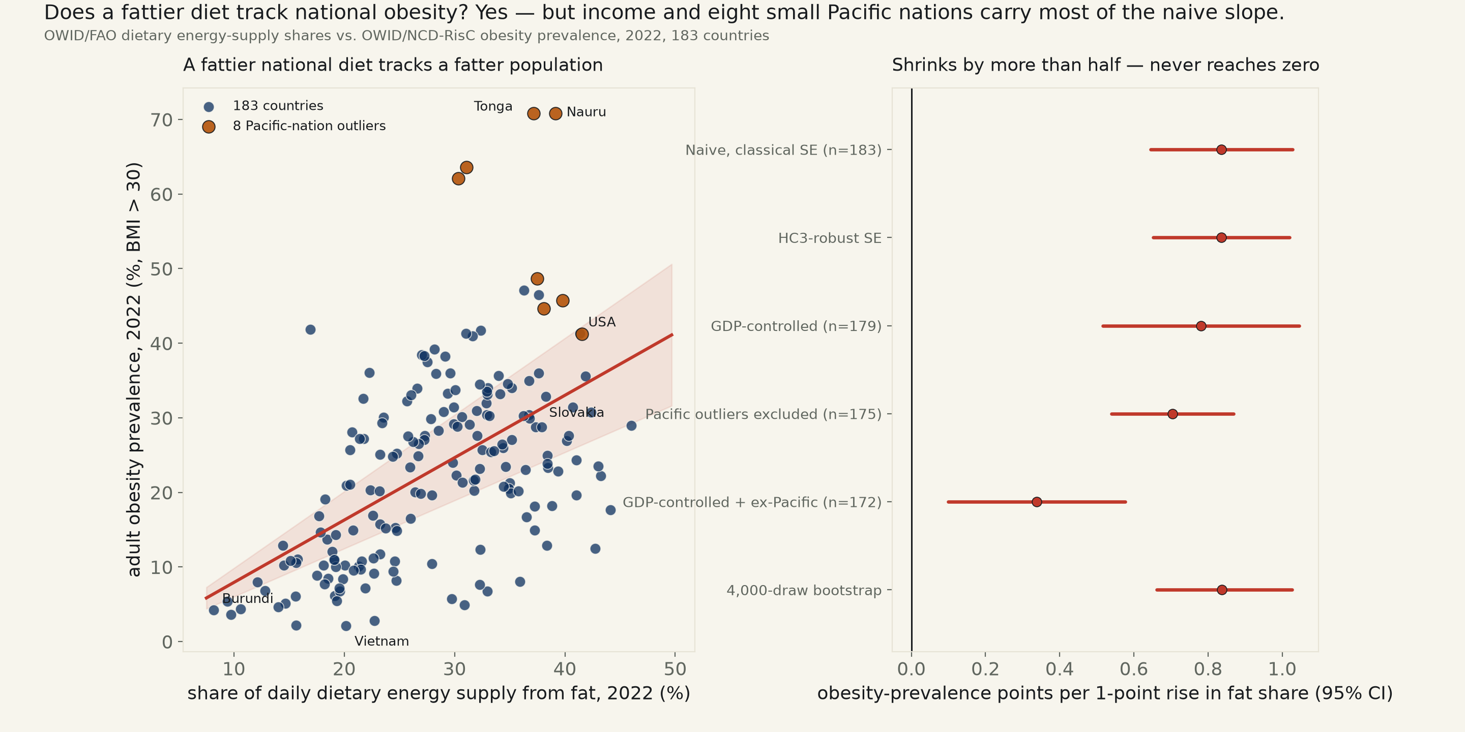
Backlog item #80, previously untouched (scoped off sugar specifically, which no OWID/FAO slug publishes standalone — see fetch_dietobesity_573.py). OWID/FAO's own share of daily dietary energy supply from fat vs. OWID/NCD-RisC/WHO's own adult obesity prevalence, 183 countries, 2022, World Bank GDP per capita (PPP) already joined by OWID in the same file. Naive OLS: +0.836 obesity-prevalence points per 1-point rise in fat share, 95% CI [+0.645, +1.027] — excludes zero, agreeing under HC3-robust SE and a 4,000-draw bootstrap (100% of resampled slopes positive). Controlling for GDP per capita alone barely moves it (+0.781, CI [+0.516, +1.045]); excluding eight small Pacific nations alone barely moves it either (+0.704, CI [+0.539, +0.869]) — but doing both at once, the strictest cut, cuts the slope to 40% of its naive size: +0.338, CI [+0.100, +0.577] — still excludes zero, a real but much smaller relationship. Tonga and Nauru, this sample's two most extreme outliers, both post obesity prevalence above 70%. Burundi posts the lowest fat share (8.2%) and a 4.2% obesity rate; Slovakia posts the highest fat share (46.0%) at 29.0% obesity. The complementary macronutrient, carbohydrate share, runs the mirror-image negative slope at every cut.
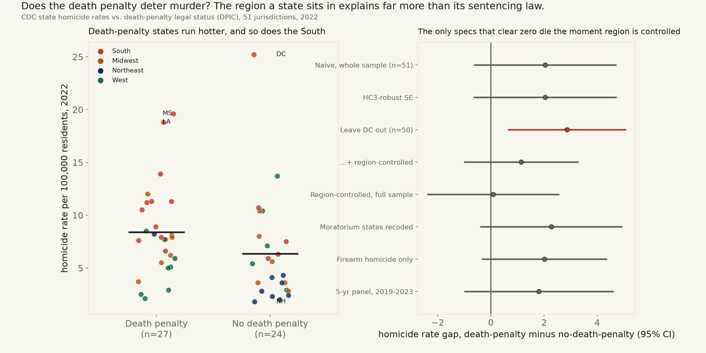
Bench idea, [NULL]-tagged: CDC's own state homicide-rate series (Mapping Injury, Overdose, and Violence, keyless) vs. death-penalty legal status (Death Penalty Information Center), 51 jurisdictions, 2022. Naive OLS runs backward for a deterrence story — death-penalty states average +2.04 more homicides per 100,000 residents, 95% CI [−0.61, +4.70] — contains zero. Drop the District of Columbia, this sample's single largest outlier and not a state, and the gap widens to +2.86, CI [+0.66, +5.07] — excludes zero, the wrong direction for the claim. But death-penalty states cluster heavily in the South, which runs structurally hotter on homicide for reasons that have nothing to do with sentencing law: controlling for Census region alone explains 36.7% of the variance, and collapses both the full-sample slope (+0.09, CI [−2.38, +2.55]) and the DC-excluded one (+1.14, CI [−0.99, +3.27]) back to a clean null. Holds recoding the 4 states under an active execution moratorium as non-death-penalty, on a firearm-only homicide rate, and across a 5-year state-clustered panel, 2019-2023.
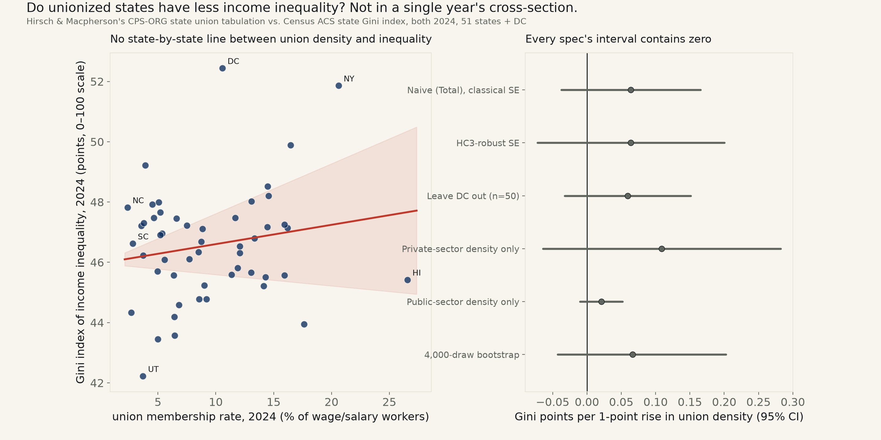
Backlog item #34, previously untouched. Hirsch & Macpherson's own CPS-ORG state union tabulation (unionstats.com) vs. the Census Bureau's own ACS Gini Index of Income Inequality (table B19083, re-served keyless via DataUSA), both 2024, 50 states + DC. Naive OLS runs the wrong direction for the claim: +0.064 Gini points per 1-point rise in union density, 95% CI [−0.037, +0.165] — contains zero, and agrees under HC3-robust SE, a Spearman rank correlation, and dropping DC. Isolating private-sector density — the sector collective-bargaining theory actually names as compressing wages — doesn't rescue the claim either: +0.109, CI [−0.064, +0.282], still contains zero; public-sector density alone is the tightest of any spec and still contains zero. Utah has the nation's lowest Gini (42.2) at a below-median union rate (3.7%); Hawaii has the single highest union rate in the country (26.6%) and an almost exactly average Gini (45.4).
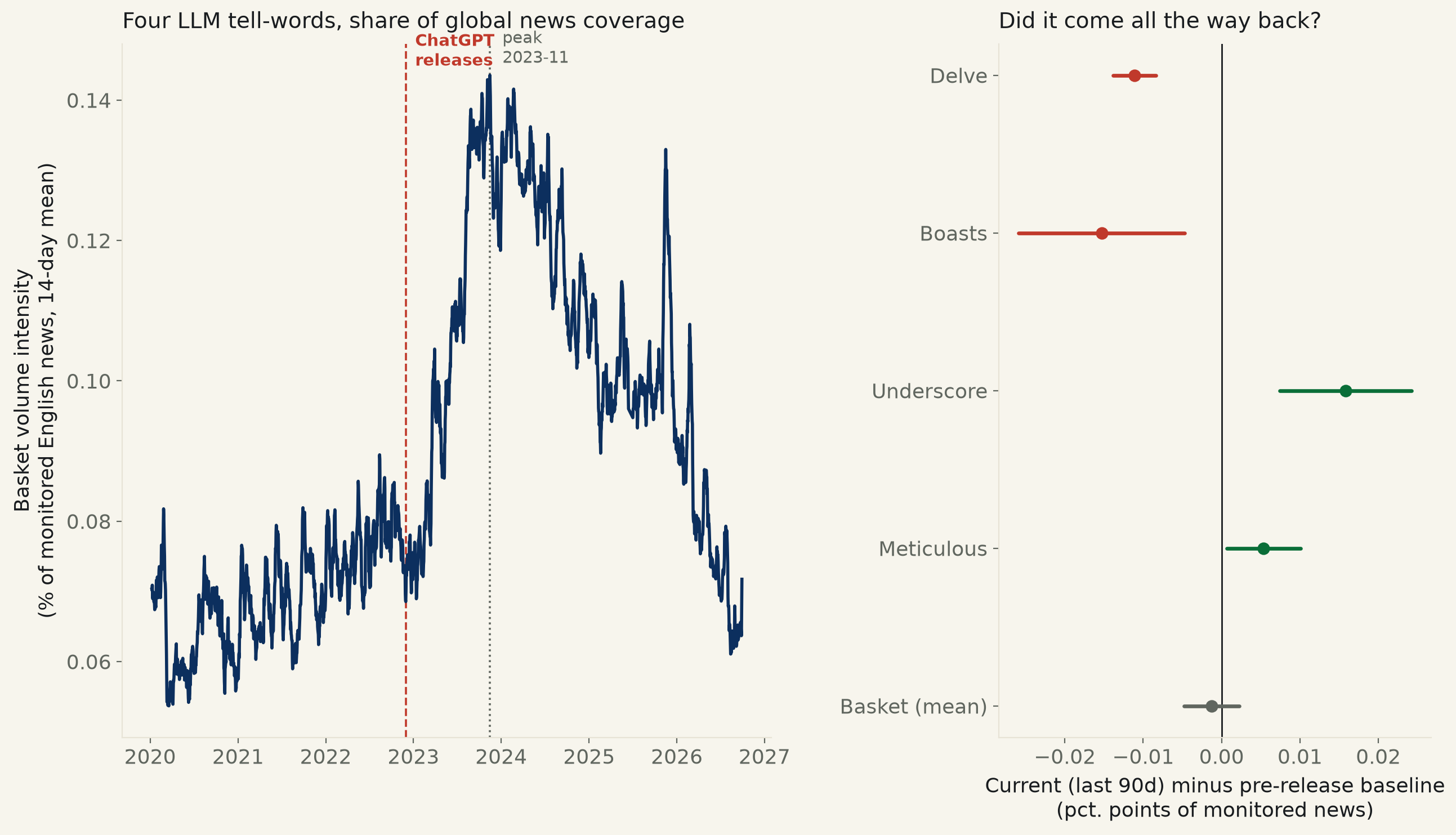
Backlog item #105, extending run 023's arXiv finding to published journalism: GDELT's own daily “Volume Intensity” (% of all monitored global English-language news mentioning a term) for four LLM tell-words — delve, boasts, underscore, meticulous — 2,440 days, 2020-01-01 to 2026-10-10, keyless. All four rose after ChatGPT's 2022-11-30 release (release-to-peak slope excludes zero for every word, basket +0.081 pts/yr, CI [0.073, 0.088]), peaking basket-wide at 1.94× baseline in Nov 2023. Three years on, the basket looks fully recovered (current vs. pre-release baseline, CI [−0.0048, +0.0022] — contains zero) — but that average hides a split: delve now sits 31% BELOW its own pre-ChatGPT baseline (CI excludes zero) and boasts 10% below, while underscore is still 30% above baseline and meticulous 16% above (both CIs exclude zero, the wrong direction for a 'funeral'). The aggregate's apparent null is two overshoots cancelling two residues, not four words behaving alike.
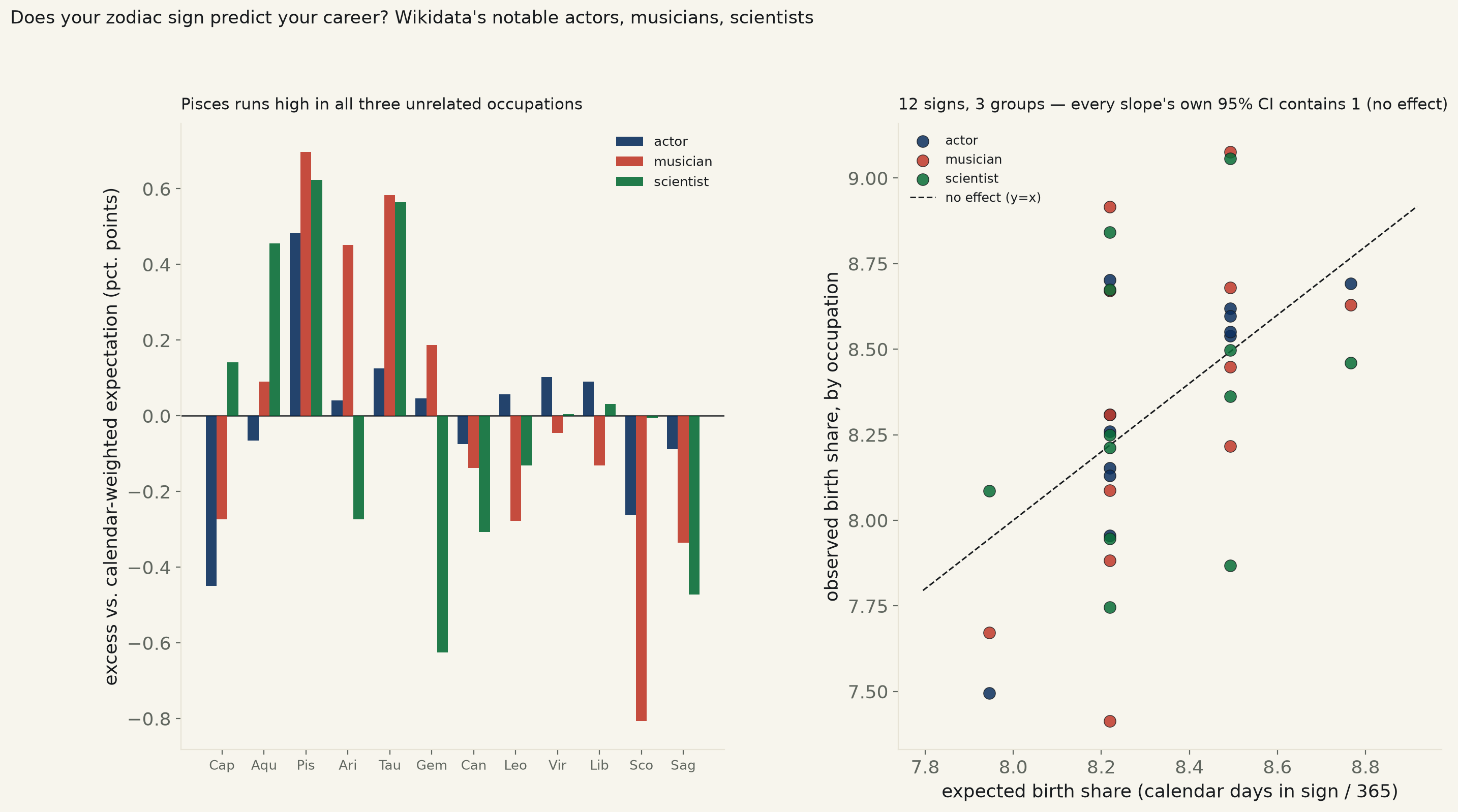
301,720 Wikidata people with a day-precision birth date (213,363 actors, 66,926 musicians, 21,431 scientists), live SPARQL pull, a known January-1 placeholder-date artifact excluded by construction. Naive chi-square goodness-of-fit against a calendar-day-weighted null "rejects" in all three groups — p=4.3×10⁻²⁶ (actors), 2.2×10⁻²⁹ (musicians), 5.9×10⁻⁶ (scientists) — but every single sign's deviation tops out under 0.8 percentage points; at N in the hundreds of thousands, the chi-square has power to flag noise. Rebuilt as the regression this desk actually reports — observed birth share vs. expected birth share across the real 12 independent sign-categories — no group's slope can rule out 1 (no effect): actors 1.33, 95% CI [0.64, 2.03]; musicians 1.23, CI [−0.15, 2.62]; scientists 0.50, CI [−0.74, 1.74]. The one thing all three unrelated occupations agree on: Pisces runs the highest excess share in every group, and actors' and musicians' full 12-sign excess fingerprints correlate with each other, r=0.72, p=0.008 — astrology doesn't predict that two unrelated careers share a sign bias; a demographic quirk in Wikidata's own notable-people pool does.
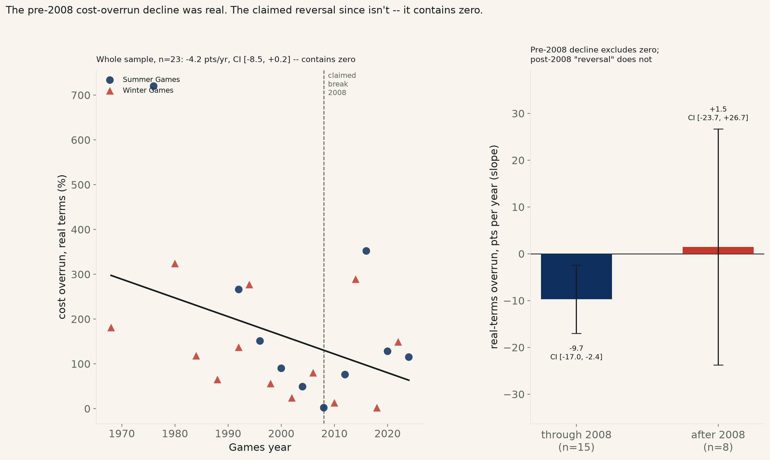
23 Olympic Games, 1968–2024, real-terms cost overrun (%), Table 4 of Budzier & Flyvbjerg's Oxford Olympics Study 2024 (arXiv:2406.01714), fetched and parsed live from the paper's own PDF. That paper's abstract claims overruns "were decreasing until 2008, but have increased since then." The first half holds: through 2008 (n=15), slope −9.7 points/year, 95% CI [−17.0, −2.4] — excludes zero. The second half doesn't: after 2008 (n=8), slope +1.5 points/year, 95% CI [−23.7, +26.7] — contains zero, indistinguishable from flat, and an interaction test asking whether the slope actually changed between eras also contains zero (p=0.35). Even the whole-sample real-terms trend across all 23 Games, −4.2 points/year, sits a hair from the standard threshold, CI [−8.5, +0.2], p=0.059.
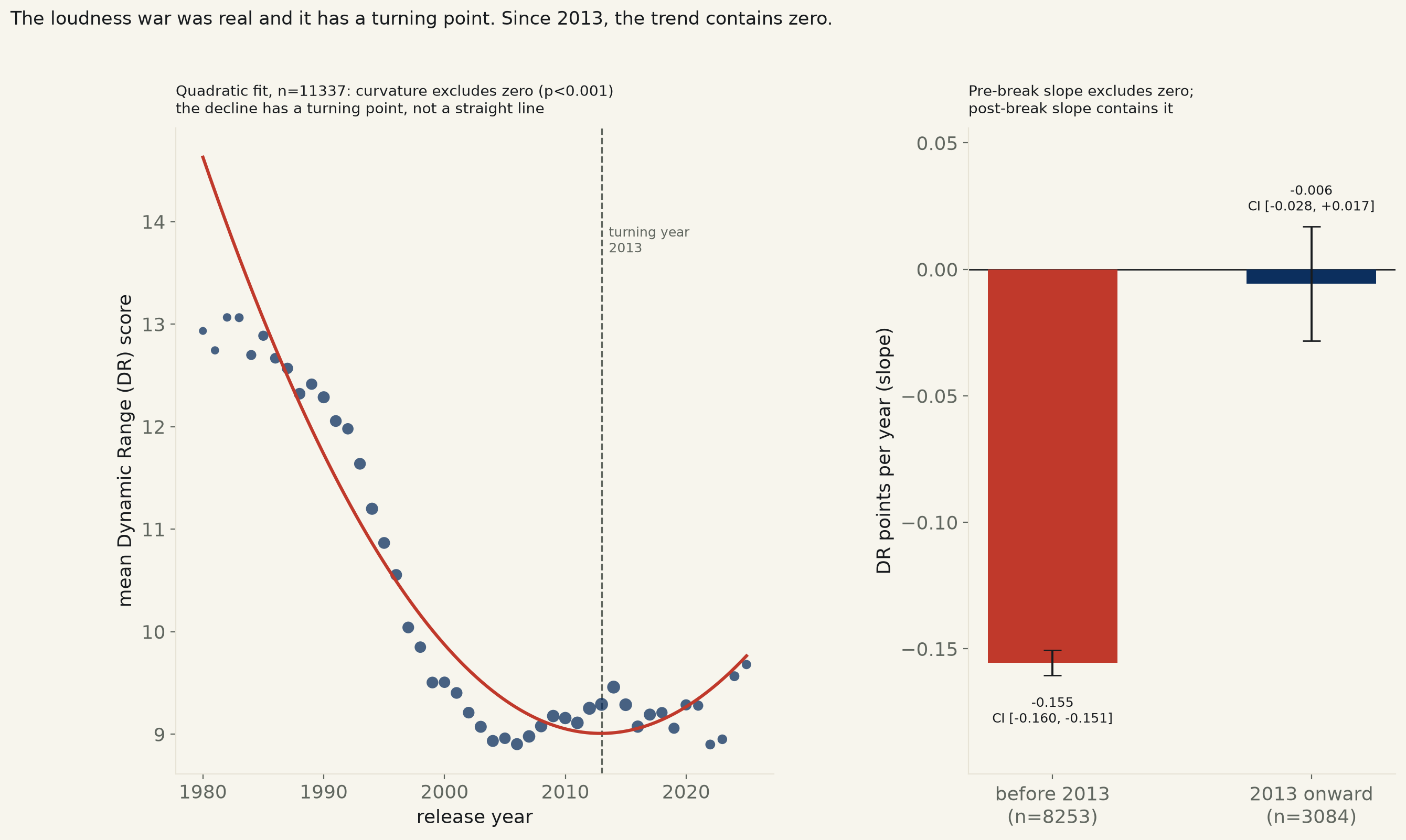
11,337 albums (1980–2025), a systematic artist-alphabetical sample of the crowdsourced Dynamic Range Database's ~194,000 entries, scraped live and keyless. Naive linear fit: Dynamic Range falls −0.101 points per year, 95% CI [−0.105, −0.098], p<0.001, R²=0.22 — the loudness-war claim, confirmed in direction. But a quadratic term fit to the same data finds real curvature (CI on the quadratic coefficient excludes zero) with a turning point at 2013, not hand-picked: before 2013, slope −0.155 points/year, CI [−0.160, −0.151], excludes zero; from 2013 on, slope −0.006, CI [−0.028, +0.017] — contains zero, and an interaction test confirms the slope genuinely changed, not just noise around one number. The loudness war bottomed out and stalled; it did not reverse, and it did not continue.
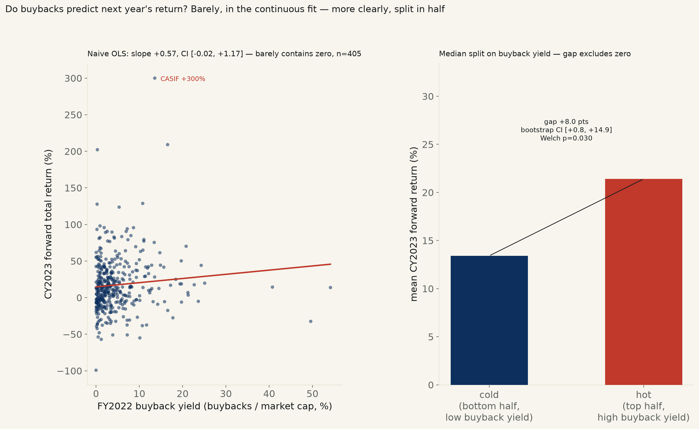
405 US-listed operating companies, SEC XBRL frames (keyless) for FY2022 buybacks and shares outstanding, joined to yfinance prices. Naive OLS: every extra point of FY2022 buyback yield tracks with +0.57 points of CY2023 forward return, 95% CI [−0.02, +1.17], p=0.059 — barely contains zero, and the near-miss is one stock: drop the single most extreme return in the sample (CASI Pharmaceuticals, +300%) and the CI widens to [−0.15, +0.96]. A rank-based measure immune to that one outlier, Spearman's ρ=0.153, p=0.002, says the same ordering holds anyway and survives dropping the top 3 extreme returns. Split the same 405 companies at the median buyback yield into heavy vs. light buybackers: heavy buybackers averaged +21.4% the next year against light buybackers' +13.4%, a +8.0-point gap, 95% bootstrap CI [+0.8, +14.9] — excludes zero. Controlling for company size leaves it contained in zero again.
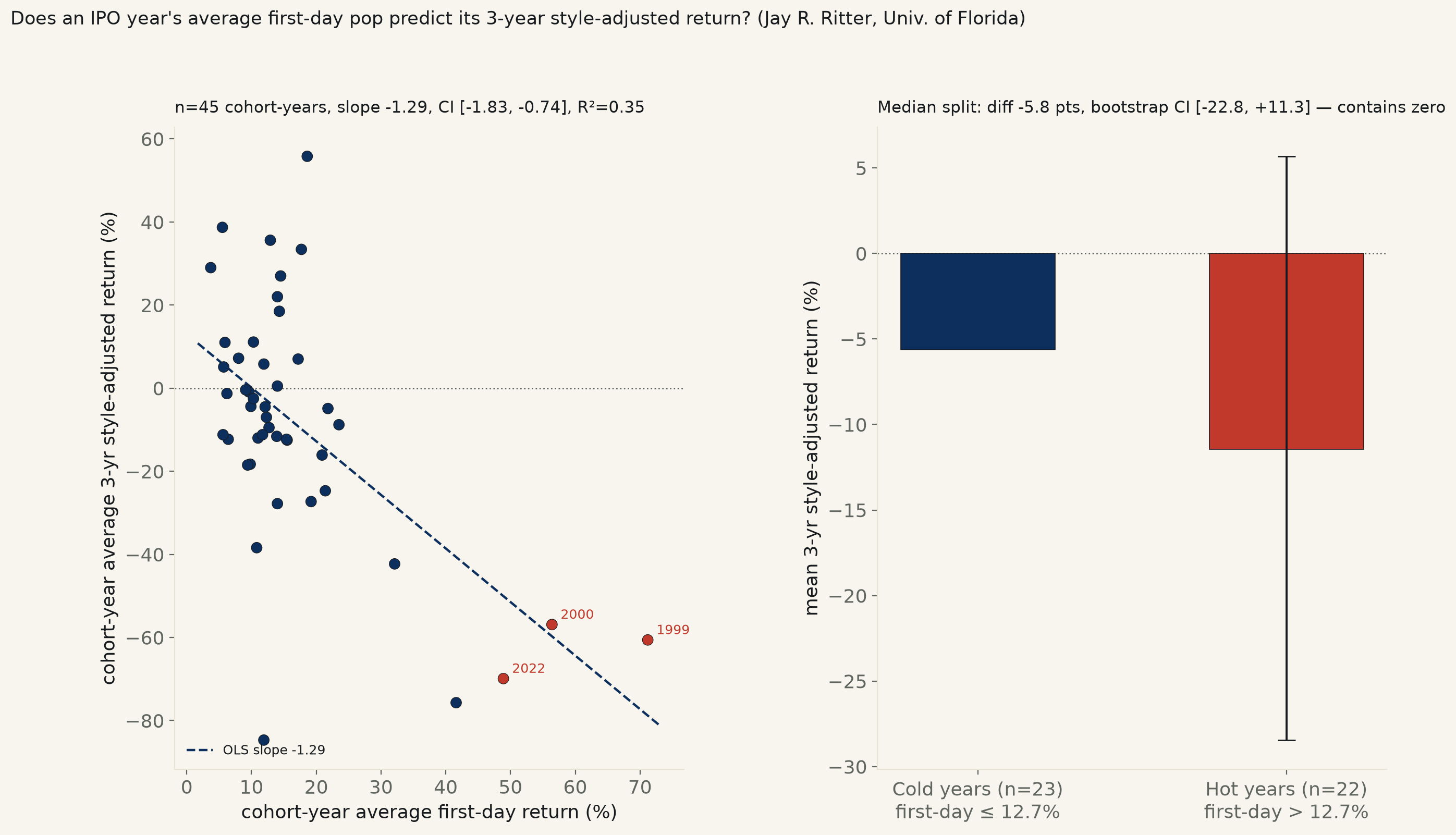
45 IPO cohort-years, 1980–2024 (9,253 IPOs total), Jay R. Ritter's (Univ. of Florida) own published annual tables, fetched live. Regressed across all 45 years, each year's average first-day return predicts that year's average 3-year style-adjusted return: slope −1.29 points of underperformance per point of extra pop, 95% CI [−1.83, −0.74], R²=0.35, p<0.001 — excludes zero, and survives dropping the two dot-com-bubble years. But split the same 45 years at the median into "hot" and "cold" halves — the backlog's own two-population framing — and the gap, −5.8 points, no longer clears zero: Welch's p=0.52, bootstrap CI [−22.8, +11.3]. The continuous relationship is real but is carried by a handful of extreme years, not a clean two-population split. Separately: IPO cohort-years underperform their size/book-to-market-matched peers in 30 of 45 years (66.7%), regardless of that year's pop.
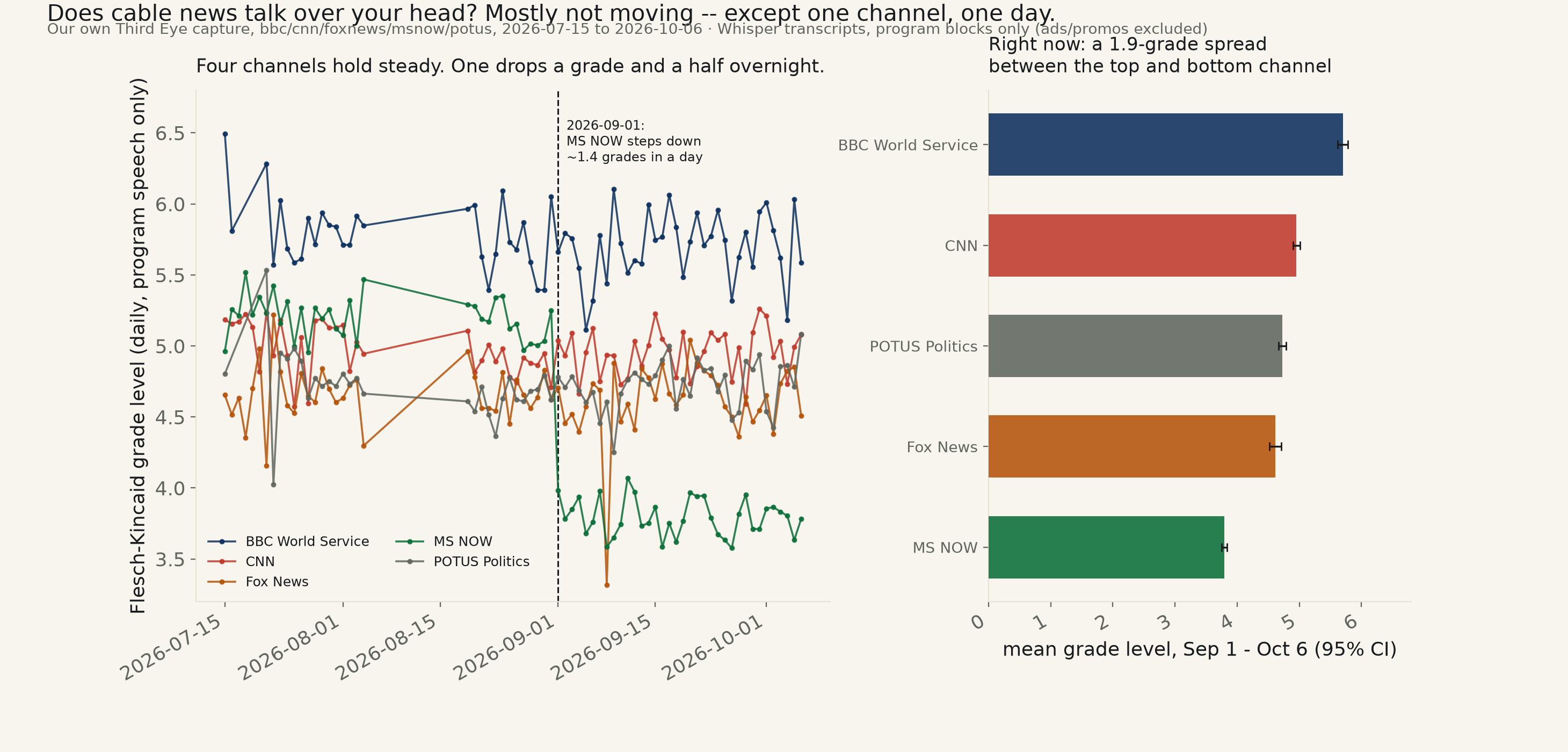
341 channel-days, our own Third Eye speech capture (bbc/cnn/foxnews/msnow/potus), Whisper transcripts of on-air program speech only, ads and promos excluded. Pooled across all five, Flesch-Kincaid grade level technically falls −0.042 grades/week, 95% CI [−0.065, −0.019] — excludes zero. But that's one channel's arithmetic wearing a trend's clothes: MS NOW holds steady around grade 5.2 through August, then drops to grade 3.8 within a single day, 2026-09-01, and stays there (−1.40 grades, 95% CI [−1.47, −1.34]). Drop MS NOW and the pooled "trend" across the other four shrinks to −0.008 grades/week, CI [−0.014, −0.001] — barely excludes zero, and only BBC's own slice of it does. CNN, Fox News, and POTUS Politics show no trend in either direction. Right now, BBC runs a full 1.9 grades above MS NOW, the widest gap in the capture.
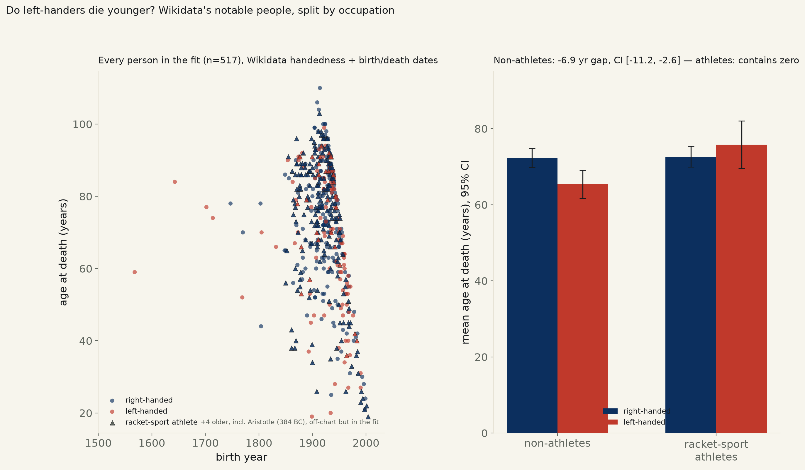
517 people (133 left-handed, 384 right-handed), Wikidata's own handedness + birth/death-date statements, live SPARQL pull. Naive: left-handed people in this sample die 4.74 years younger on average, 95% CI [−8.39, −1.08], p=0.011 — excludes zero, and a 4,000-draw bootstrap agrees. The textbook explanation for the 1988 Coren & Halpern finding is a birth-cohort artifact (older generations under-report left-handedness); adding birth year as a control barely moves the gap, −5.01 years, CI [−8.68, −1.33]. Wikidata's own handedness statements are dominated by racket-sport athletes (224 of 517, mostly tennis and badminton, where “handedness” often just means playing hand) — split them out and the gap flips null among athletes (CI [−4.2, +10.43], contains zero) and gets bigger among everyone else (−6.89 years, CI [−11.22, −2.56], bootstrap agrees).
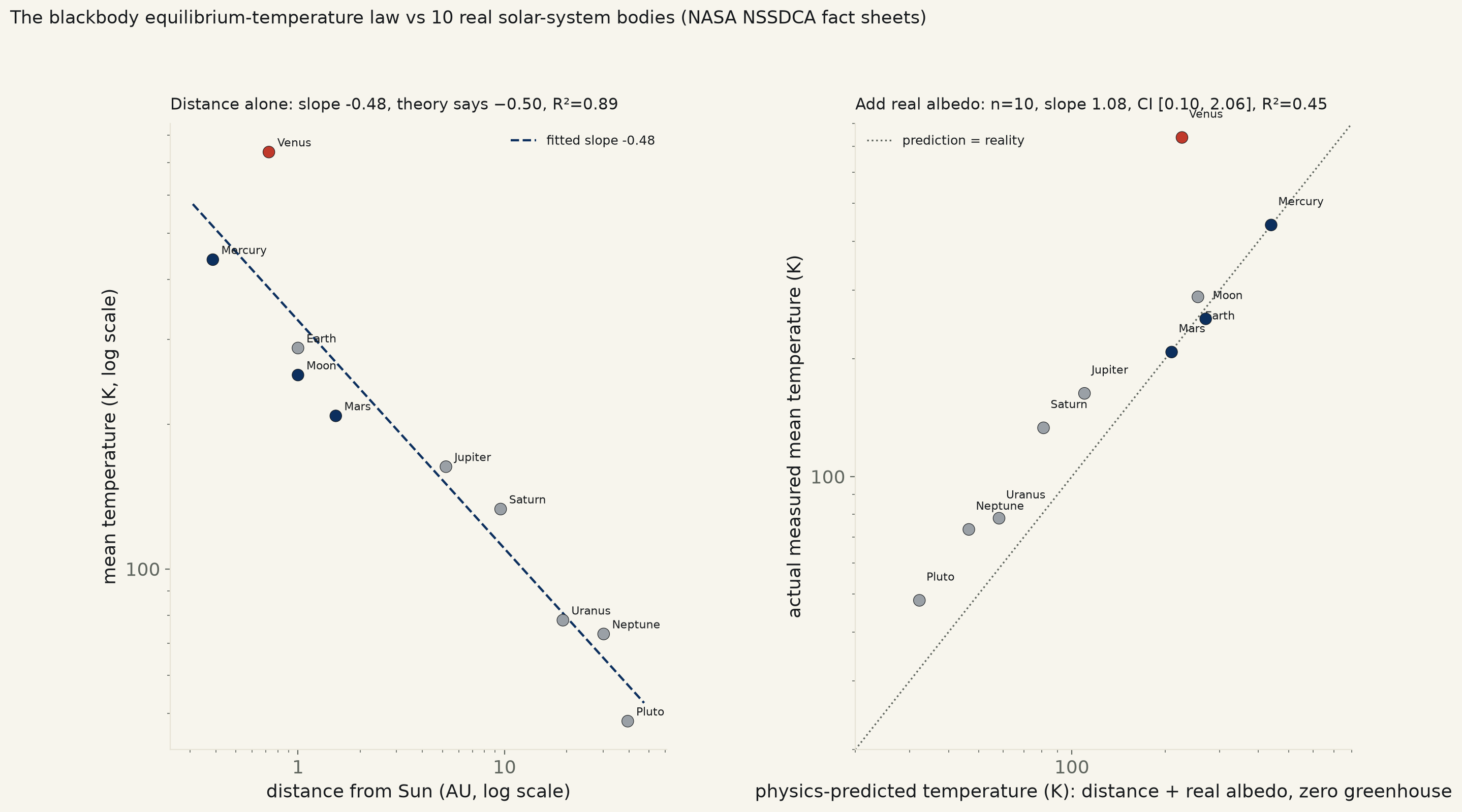
10 solar-system bodies (8 planets, the Moon, Pluto), NASA NSSDCA Planetary Fact Sheets, fetched live — distance, mean temperature, and each body's own Bond albedo. Distance alone predicts temperature with slope −0.48 (theory: −0.50), R²=0.89. Add real albedo and regress actual temperature on the full physics prediction across all 10: slope +1.08, 95% CI [0.10, 2.06], R²=0.45, p=0.034 — technically excludes zero but barely informative, because Venus alone runs +510 K hotter than predicted. Drop Venus: slope 0.91, CI [0.77, 1.04], R²=0.97, n=9 — prediction equals reality for the other nine. Gas giants (internal heat) and Earth (a real, much smaller greenhouse effect) run modestly warm; airless Mercury, the Moon, and Mars land within 2 K of the line.
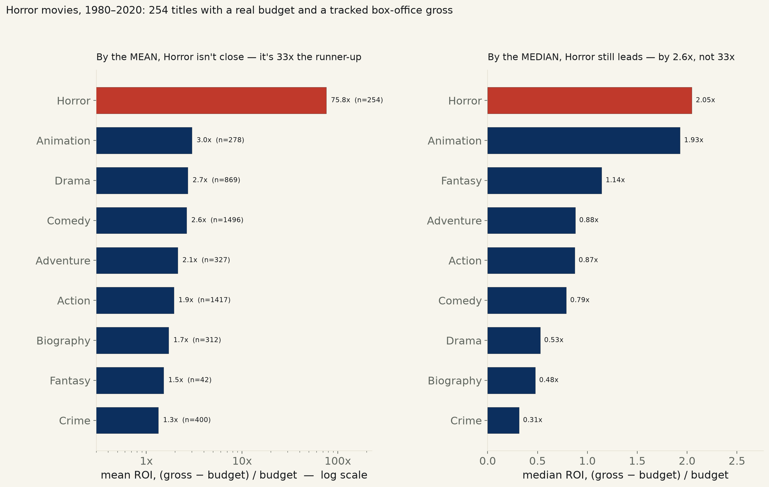
5,436 films, 1980–2020, with a real budget AND a tracked worldwide gross on file (danielgrijalva/movie-stats, a keyless GitHub mirror of an IMDb scrape — TMDB, the source IDEAS.md named, needs a key not on file). Horror's raw mean ROI is 75.8x, 33 times the next genre's 2.3x — and one film from collapsing: drop Paranormal Activity (budget $15,000, gross $193M) and it falls to 25.1x. Regressed in log space instead, log(1+ROI) on a Horror indicator: slope +0.71, 95% CI [0.48, 0.93], R²=0.011, n=5,436, p<0.001 — excludes zero, geometric-mean ROI 200% vs 48%, a 4.2x gap. The raw median gap is smaller still: 2.05x vs 0.79x, 2.6x. Three honest lenses, three different magnitudes, same direction.
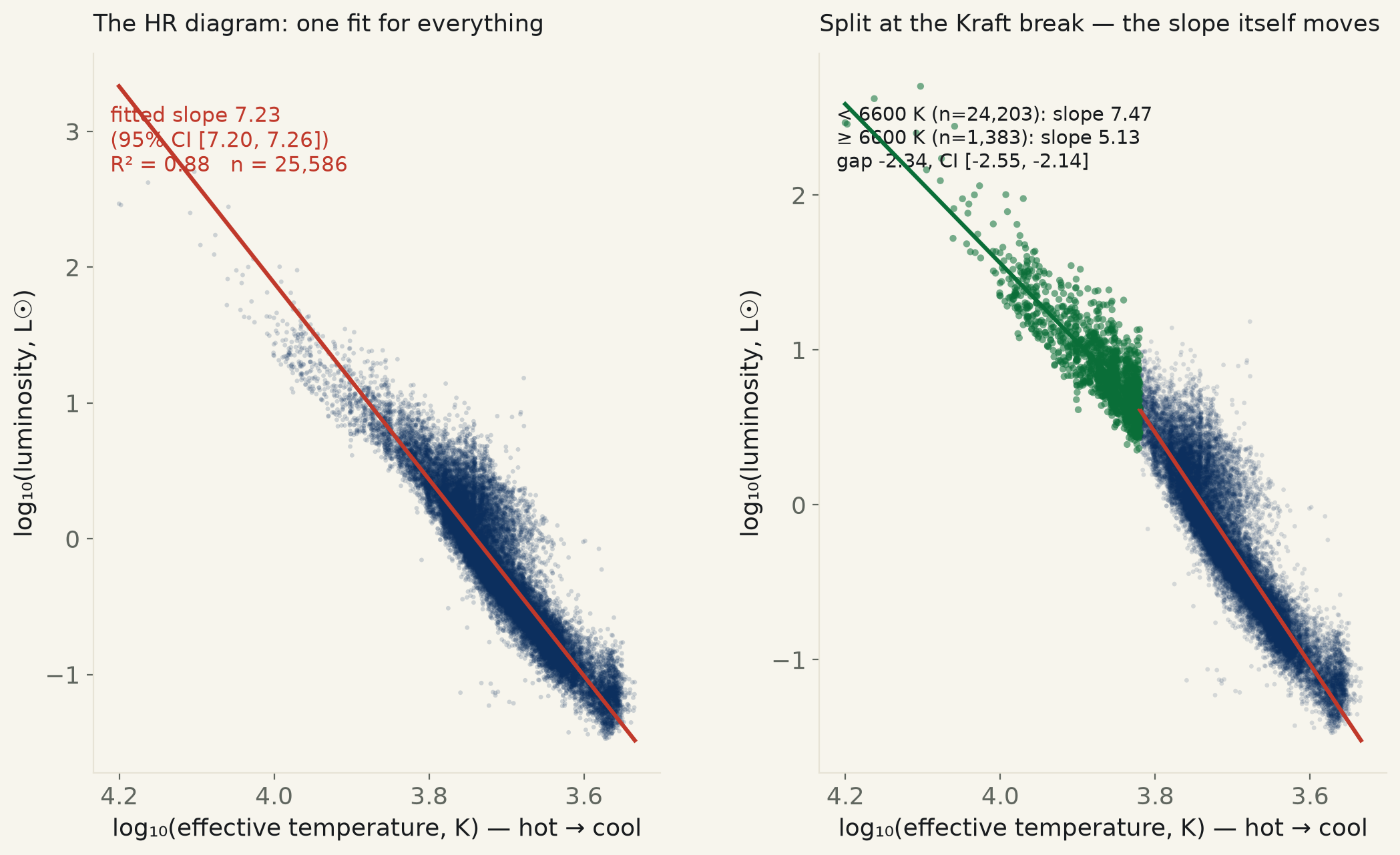
25,586 main-sequence dwarf stars, Gaia DR3 astrophysical_parameters (GSP-Phot temperature, FLAME luminosity/radius), keyless TAP sync. Whole-sample log(luminosity) on log(temperature): slope 7.23, 95% CI [7.20, 7.26], R²=0.88. Split at 6600 K, the Kraft break separating convective-envelope from radiative-envelope dwarfs: slope 7.47 below (n=24,203) vs 5.13 above (n=1,383) — a gap of −2.34, 95% CI [−2.55, −2.14], excludes zero. A Stefan-Boltzmann self-consistency check (temperature + radius predicting luminosity) lands at slope 1.0023, R²=0.998, but that is the same pipeline's own outputs agreeing with itself, not an independent test.
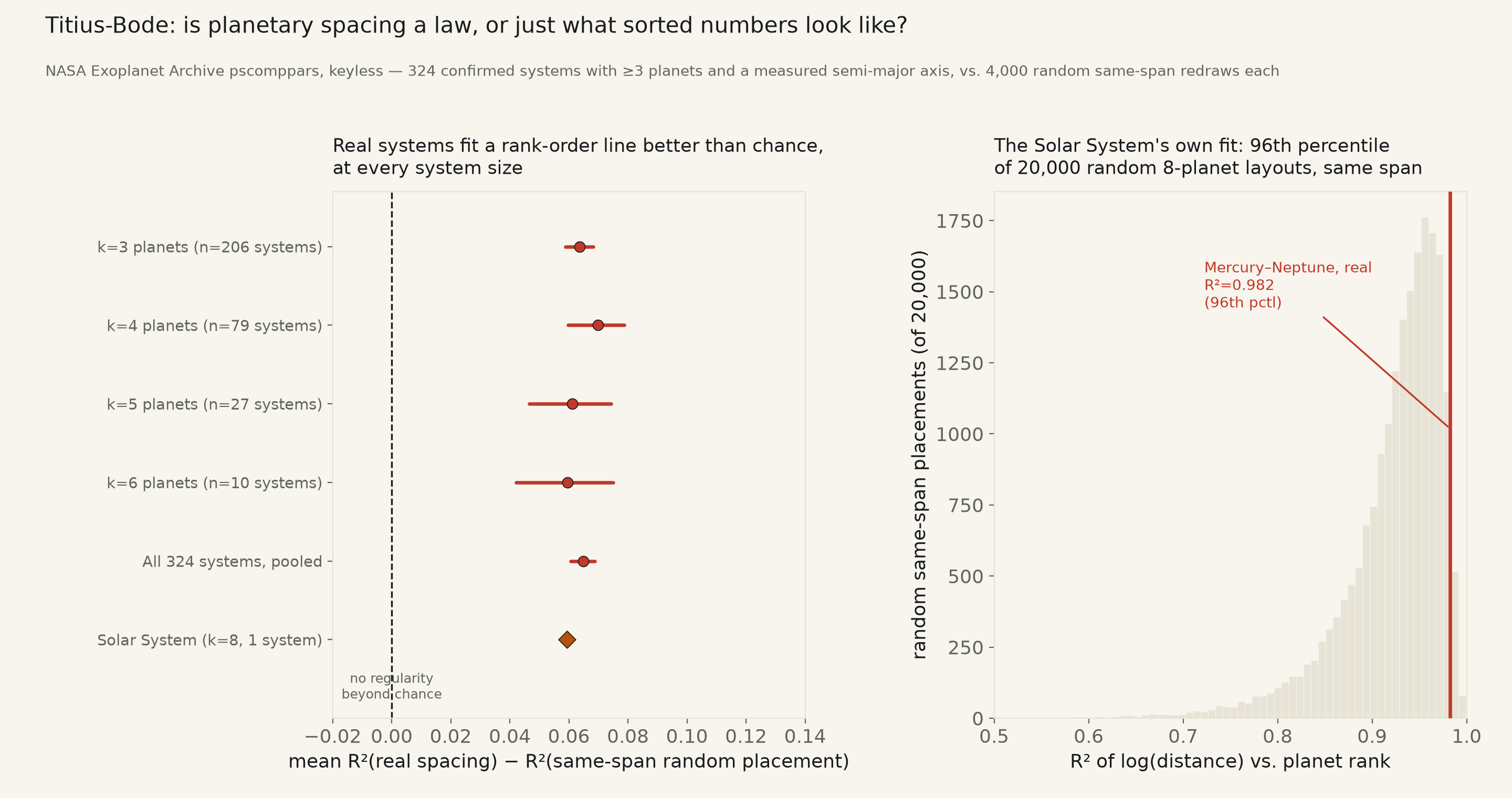
324 confirmed multi-planet systems with 3 or more planets and a measured orbital distance (NASA Exoplanet Archive pscomppars, keyless). Each system's real log-distance-vs-rank fit (mean R²=0.969) is checked against 4,000 random same-span redraws of its own interior planets (mean R²=0.904). Mean gap +0.065 R², 95% CI [0.061, 0.069] — excludes zero by a wide margin, p≈5×10−101, and holds at every system size from 3 to 6 planets. 23.8% of real systems land above their own null's 95th percentile, versus the 5% chance alone predicts. The Solar System's own Mercury–Neptune fit, R²=0.982, sits at the 96th percentile of its own 20,000-draw null — real, but not proof of the specific 1766 doubling formula Titius and Bode proposed.
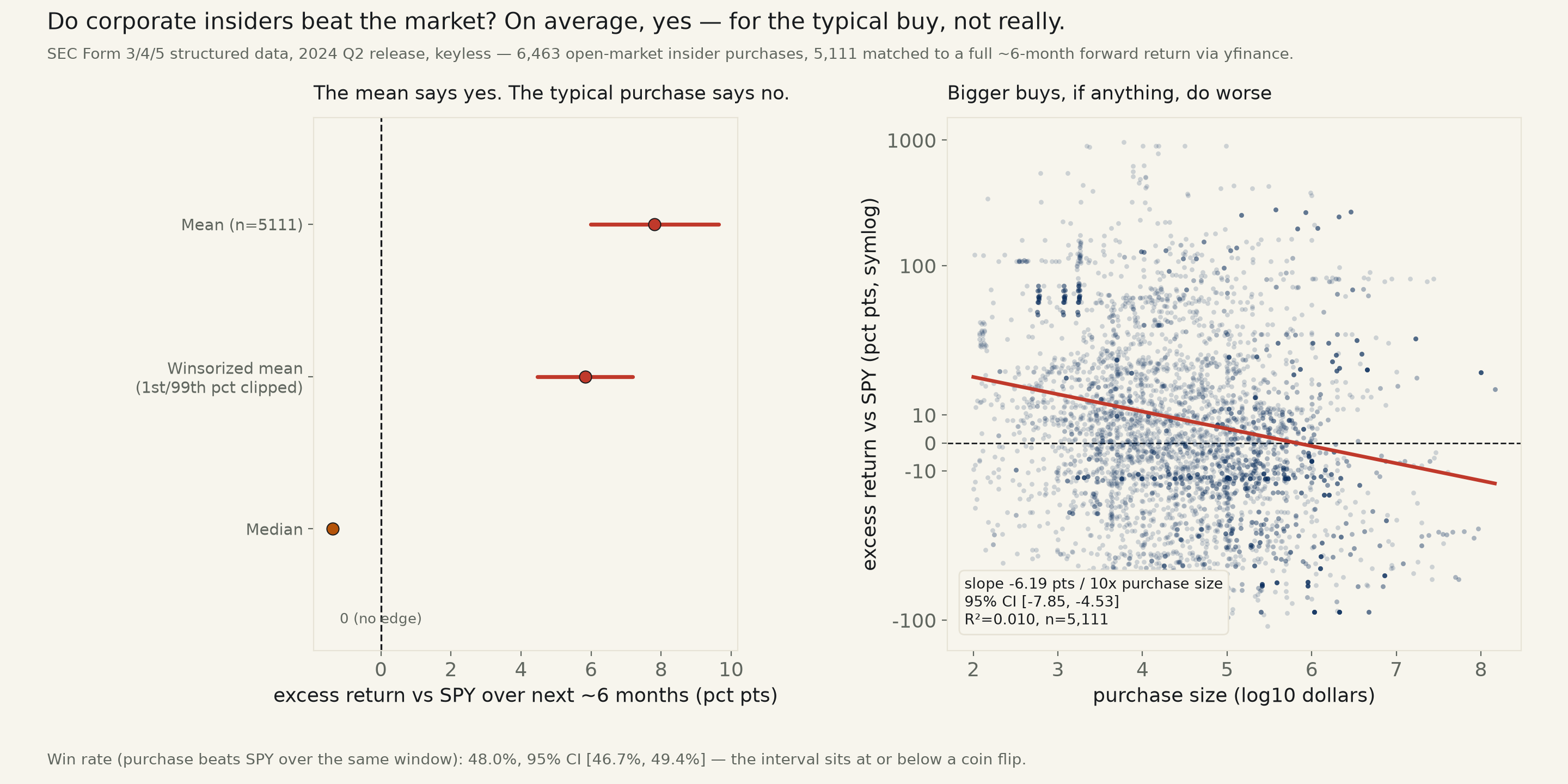
6,463 open-market insider purchases from SEC Form 3/4/5's own keyless structured data set, 2024 Q2 filings, matched to a ~6-month forward return vs SPY for 5,111 of them via yfinance. Mean excess return +7.8 points, 95% CI [6.0, 9.6] — excludes zero, and survives 1st/99th-percentile winsorizing (+5.8, CI [4.5, 7.2]). But the median purchase is −1.4 points and the win rate is 48.0%, 95% CI [46.7%, 49.4%] — at or below a coin flip. The mean is carried by a fat right tail (one purchase in Power Solutions International ran +900%); the “bigger buy, bigger conviction” version of the claim runs backward, slope −6.2 pts per 10x purchase size, CI excludes zero.
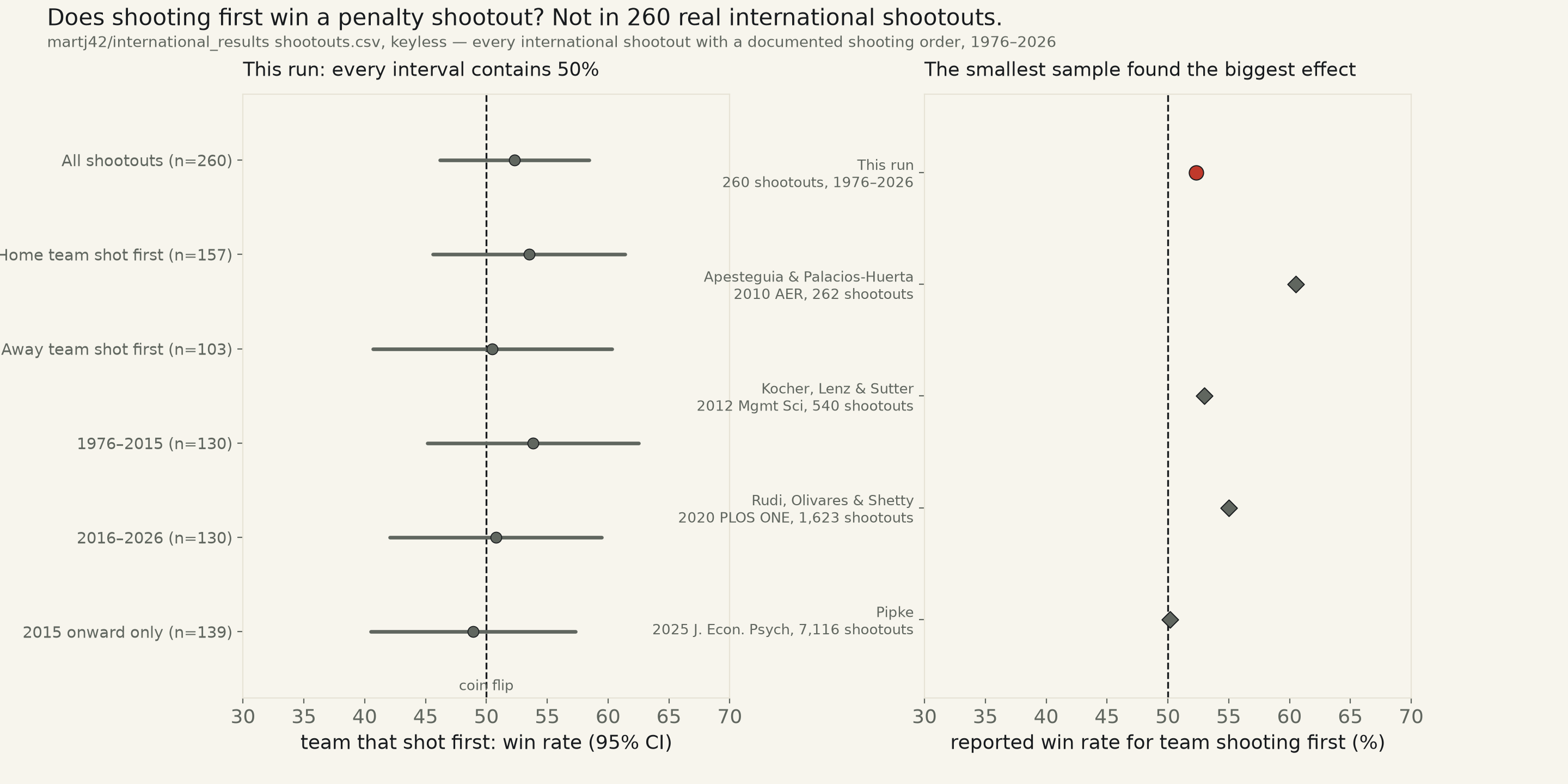
260 international shootouts with a documented shooting order, 1976–2026 (martj42/international_results, keyless). Naive: the team shooting first wins 52.3% of the time, 95% CI [46.2%, 58.4%] — contains 50%. Splitting by home/away, by era, and to 2015-onward only never clears it either. Apesteguia & Palacios-Huerta’s widely cited 2010 finding of 60.5% came from 262 shootouts; every subsequent large-sample study, and this one, lands close to 50:50.
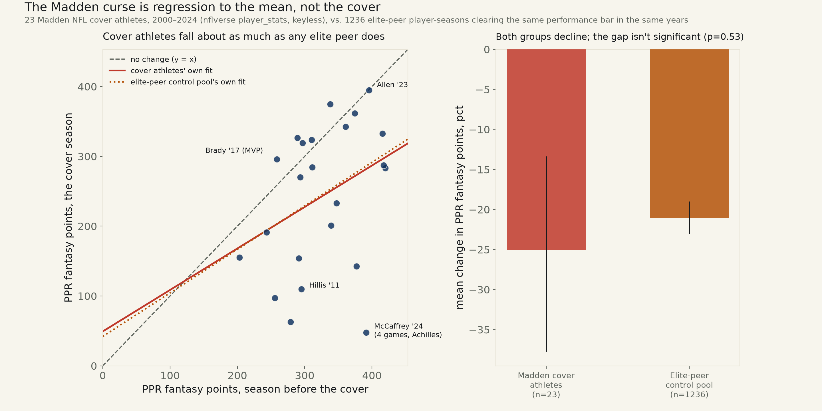
23 Madden NFL cover athletes, 2000–2024 (nflverse player_stats, keyless), vs. 1,236 non-cover player-seasons just as elite the same years. Cover athletes: −25.1% PPR fantasy points the cover season, 95% CI [−37.6%, −13.4%] — excludes zero, a real drop. Elite-peer control pool: −21.1%, CI [−22.9%, −19.1%] — also excludes zero. A Welch t-test finds no distinguishable gap between the two groups, p=0.53. Christian McCaffrey's 2024 (−87.8%, torn Achilles) is the steepest fall in the sample; Tom Brady's 2017 MVP season (+14.4%) is the steepest rise.
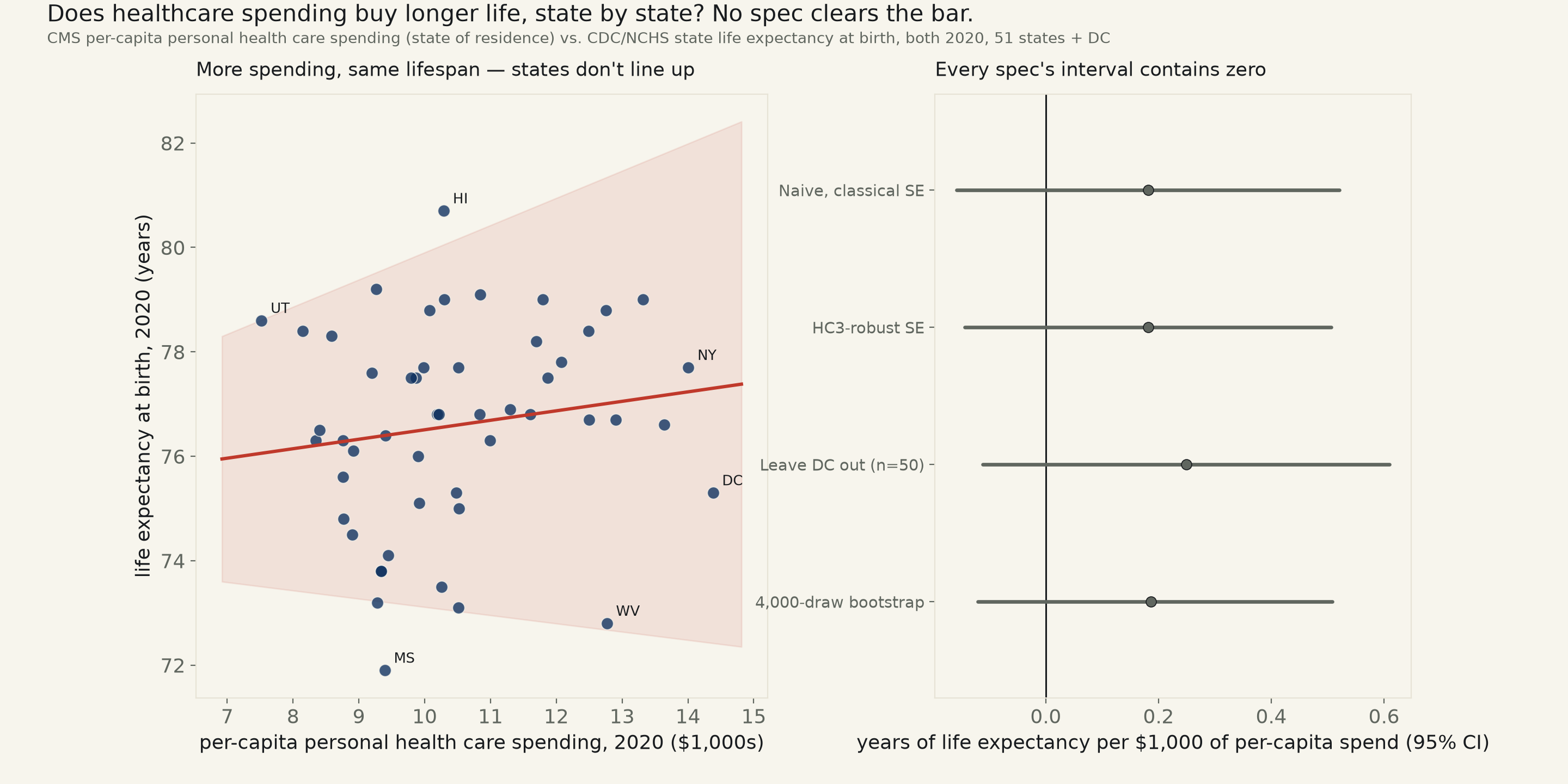
51 US states + DC, 2020: CMS per-capita personal health care spending (state of residence, keyless) vs. CDC/NCHS state life expectancy at birth (keyless). Naive: +0.182 yrs of life expectancy per $1,000 spent, 95% CI [−0.158, +0.521] — contains zero, R²=0.023, and agrees under HC3, Spearman, and a leave-DC-out refit. Utah spends least of any state and posts a life expectancy of 78.6 years; DC spends most and comes in at 75.3.
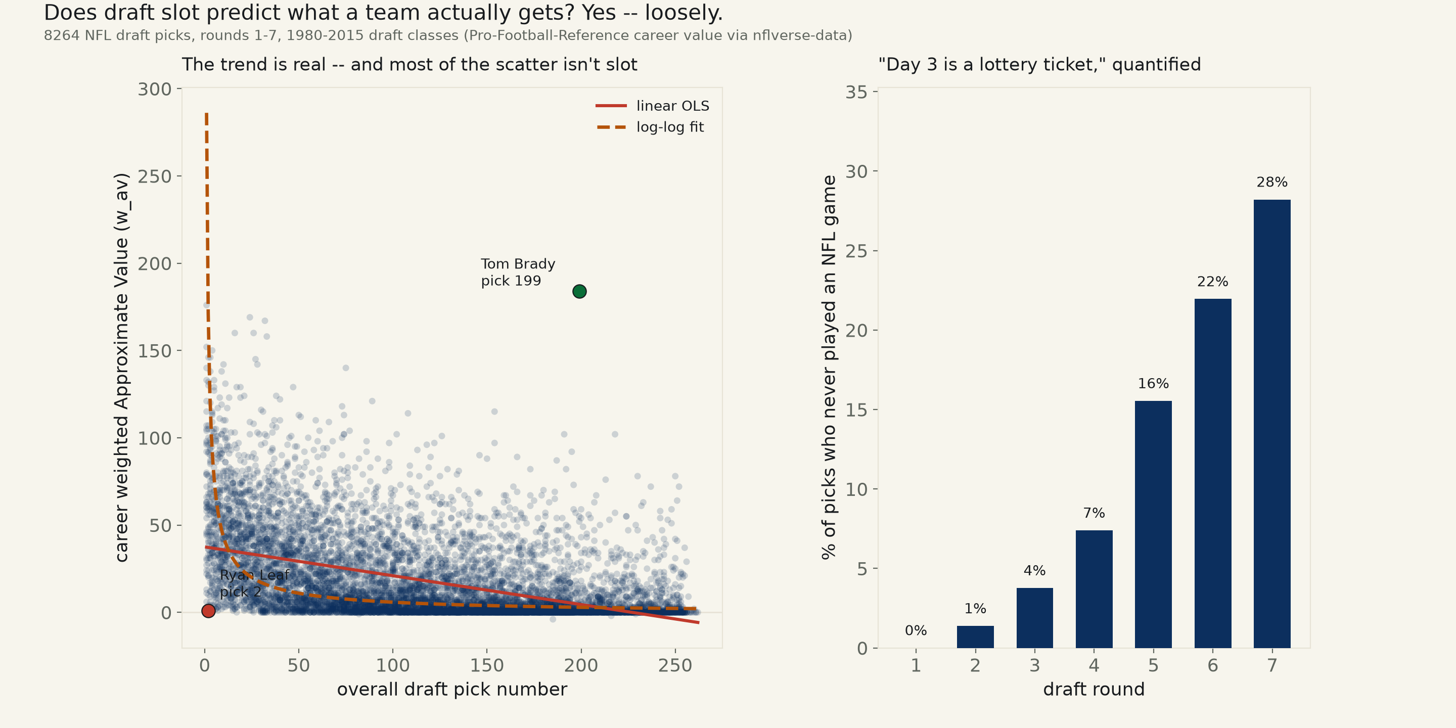
8,264 NFL draft picks, rounds 1–7, 1980–2015 draft classes, career weighted Approximate Value (Pro-Football-Reference via nflverse-data, keyless) vs. overall pick number. Naive: −0.165 career-value points per pick, 95% CI [−0.172, −0.159], p<0.001 — excludes zero, real, and a log-log curve fits even better (R²=0.275 vs 0.226) — but R² under 0.3 either way means most of any single pick's outcome isn't slot. 28% of round-7 picks never played an NFL game at all, against 0% of round 1.
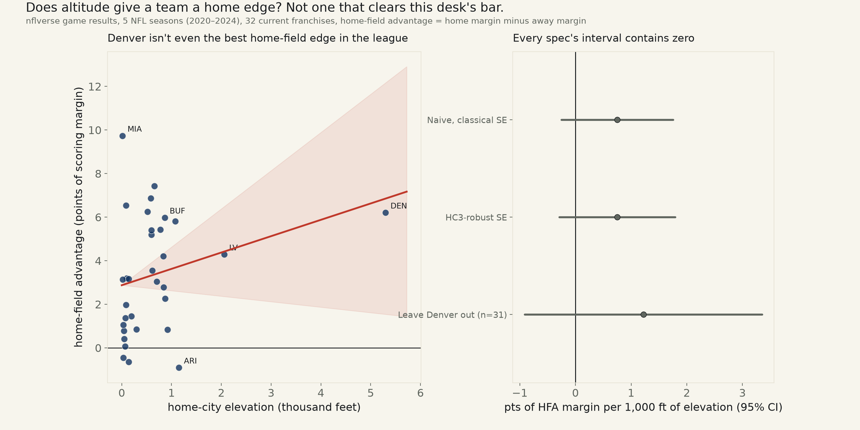
32 current NFL franchises, 2020–2024 regular seasons (the window all 32 played at their present stadium), home-field advantage (home margin minus away margin, netting out team quality) vs. real home-city elevation (nflverse game results x Open-Meteo elevation, both keyless). Naive: +0.75 pts HFA per 1,000 ft, 95% CI [−0.25, +1.75] — contains zero, and agrees under HC3, Spearman, a win-rate DV, and a leave-Denver-out refit. Denver's own HFA ranks only 6th of 32; the league's single biggest home edge belongs to Miami, at 16 feet of elevation.
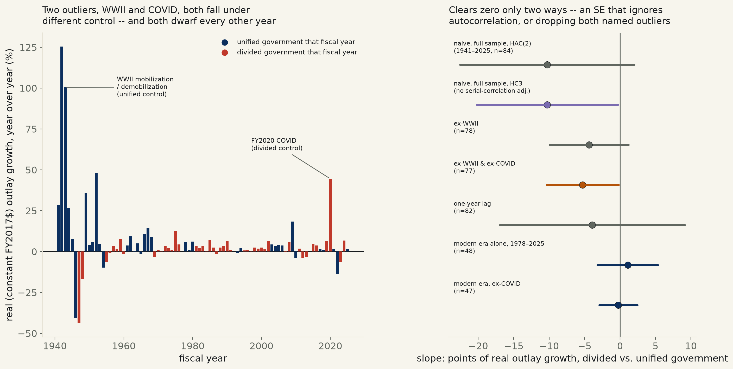
84 fiscal years, 1941–2025, real (constant FY2017$) federal outlay growth vs. a divided-government dummy (OMB's own historical outlay table x Wikipedia's party-control table). Naive, HAC-robust: −10.27 pts, 95% CI [−22.56, +2.02] — contains zero, entirely on the strength of WWII and the FY2020 COVID spike. Restricted to the modern (1978–2025) budget-process era: +1.08, CI [−3.19, +5.36] — a clean null, the opposite sign from the claim.
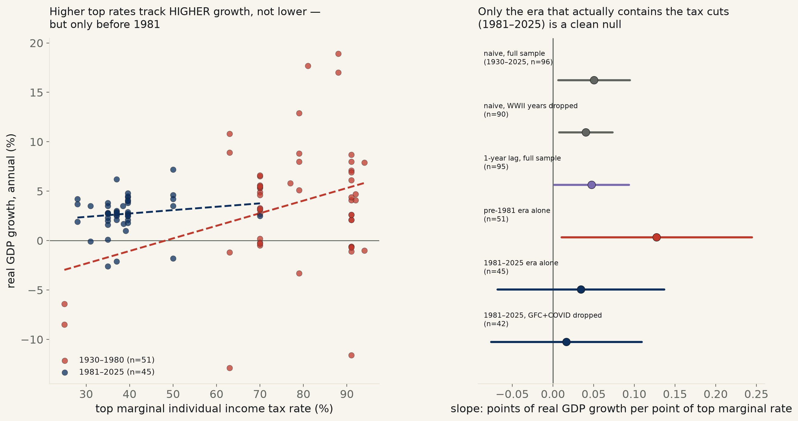
96 years, top marginal income tax rate (Tax Foundation's historical table, sourced to IRS) vs real GDP growth (BEA via FRED, keyless). Naive: +0.051 pts growth/pt rate, 95% CI [+0.006, +0.094] — excludes zero, running backward from the claim. Restricted to 1981–2025, the era that actually contains the rate cuts: +0.034, CI [−0.068, +0.137] — a clean null.
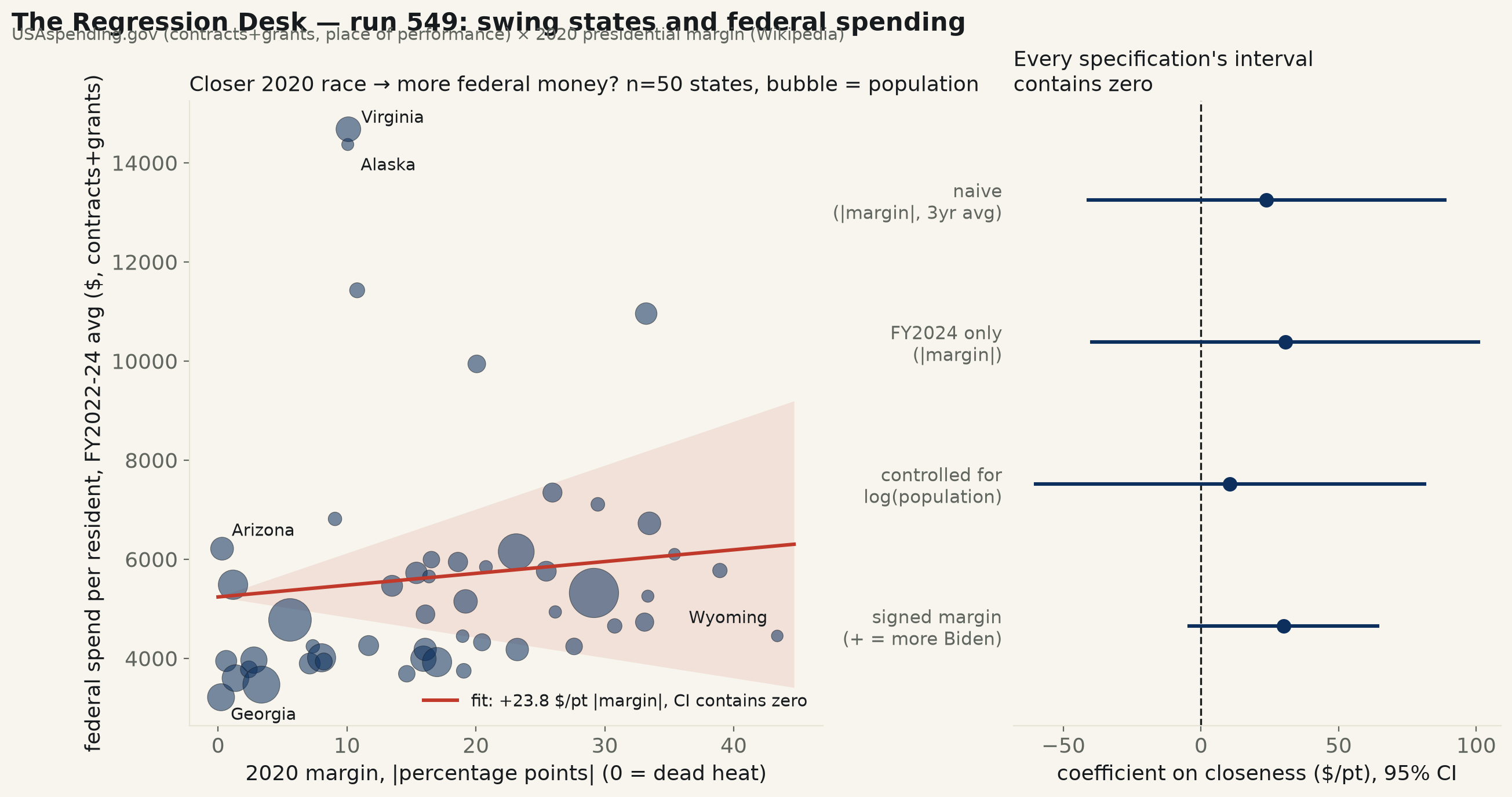
50 states, USAspending.gov contracts+grants (place of performance, FY2022–24 average, keyless) against each state's 2020 presidential margin (Wikipedia). Naive: +23.8 $/pt of |margin|, 95% CI [−40.9, +88.5] — contains zero, and the point estimate runs backward from the claim. Controlling for population, the obvious confound behind both sides of this, doesn't rescue it: still contains zero. Georgia, the single closest state in the country, has the lowest per-capita spend of all 50.
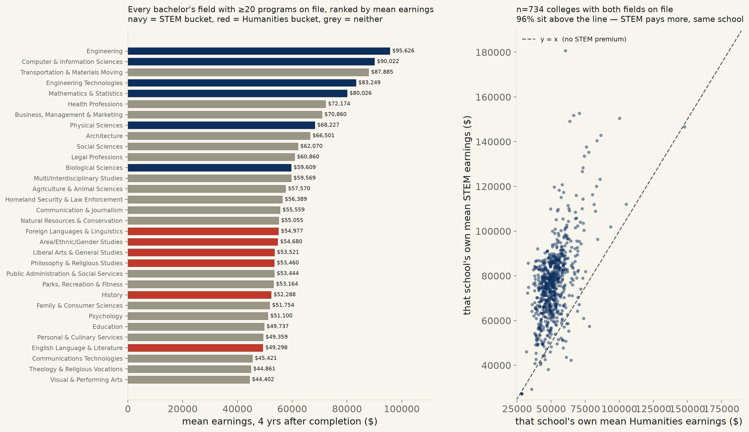
27,617 institution×major rows, bachelor's degrees only (Dept of Education College Scorecard Field-of-Study file, keyless bulk file, run 546's own stated missing variable). Naive, major-clustered: STEM programs' graduates earn $29,220 more a year than Humanities programs' graduates, 4 years after completion, 95% CI [$20,506, $37,935] — excludes zero. Compare STEM to Humanities inside the same college — holding school quality, region and selectivity fixed — and 96% of the 734 colleges with both still show STEM ahead, by $25,196 on average, CI [$24,182, $26,210].
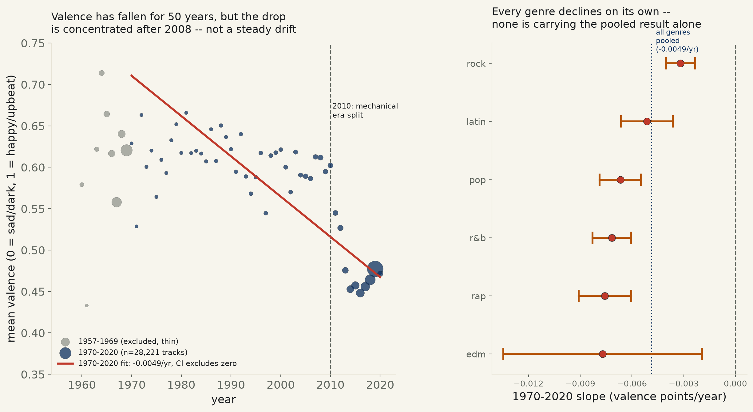
28,221 Spotify tracks, six genres, 1970–2020 (TidyTuesday, keyless). Valence — Spotify's own 0-1 “musical positiveness” score — falls -0.00486 points a year across the full record, 95% CI [-0.00557, -0.00415] — excludes zero, and every one of six genres agrees independently, from rock's shallow -0.0032/yr to edm's -0.0077/yr. A popularity-restricted robustness check (top half of each year's tracks by Spotify's own popularity score) rules out recent playlists being padded with obscure filler. But split the record at a mechanical 2010 boundary and neither era alone clears zero — only 11 independent year-clusters exist after 2010, too few to pin a single decade's rate down on its own.
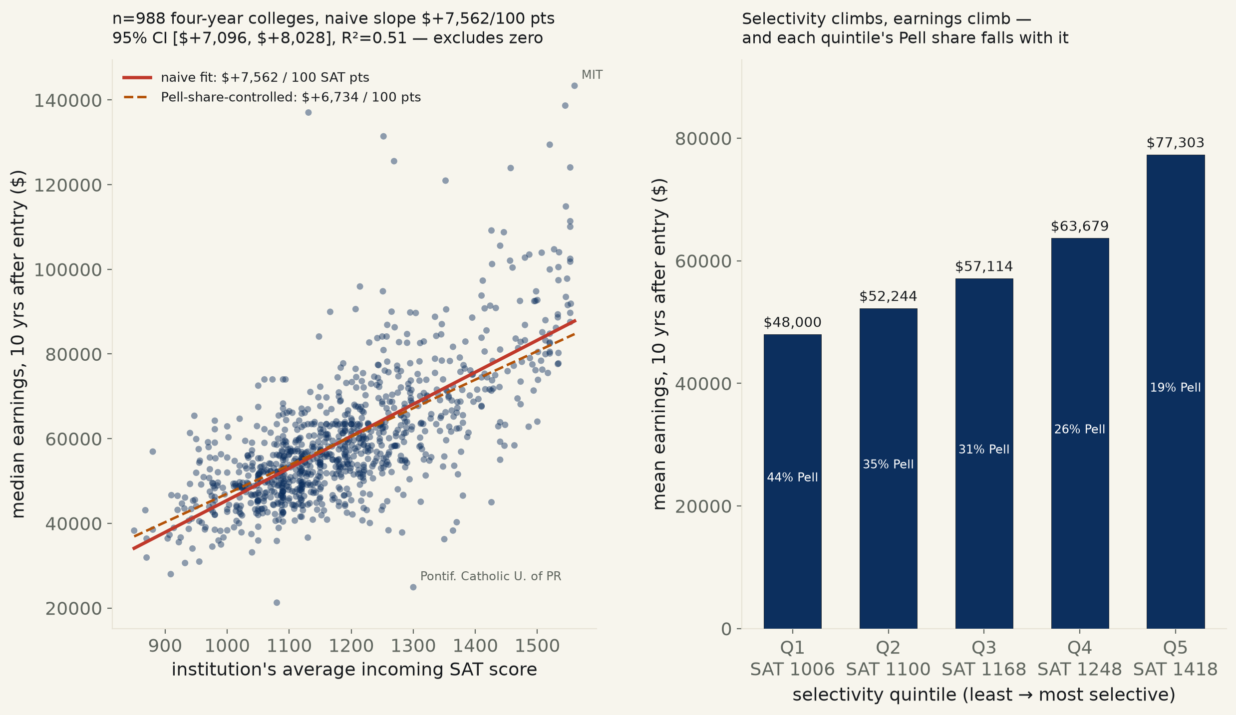
988 US four-year, bachelor's-predominant colleges (Dept of Education College Scorecard, keyless bulk file). Naive: every 100 points of an institution's average incoming SAT score tracks with $7,562 more in its graduates' median earnings 10 years after entry, 95% CI [$7,096, $8,028] — excludes zero. Add each school's own Pell-grant share (the best available institution-level stand-in for “who gets in,” since the true Dale-Krueger matched-applicant design needs individual admissions data no one publishes) and the slope barely moves, to $6,734, CI [$6,110, $7,358]. This is not that design, and the page says so: it cannot separate a school's own value-add from what its students study, the single biggest omitted confound at MIT's end of the table.
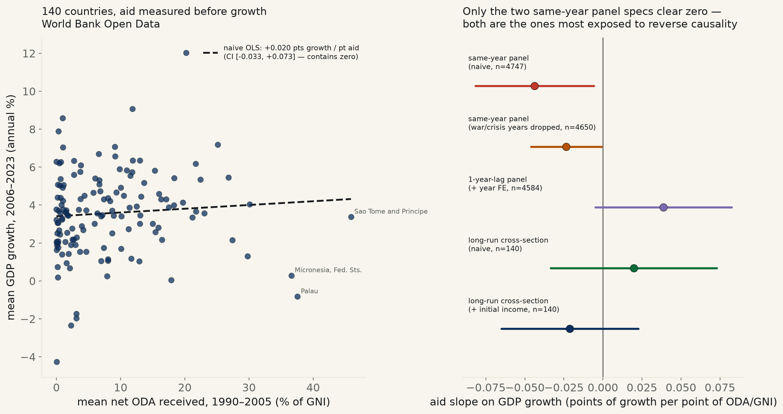
World Bank Open Data, 162 aid-recipient countries, 1990–2023. Same-year panel: every point of ODA/GNI tracks with −0.044 points less GDP growth that year, 95% CI [−0.082, −0.006] — excludes zero, but this is aid arriving during wars and collapses (Iraq 1991, Rwanda 1994), not evidence aid causes them. Lag aid by one year and the sign flips positive, CI [−0.005, +0.082] — contains zero. The design the actual aid-effectiveness literature uses — aid received 1990–2005 against growth 2006–2023, 140 countries — finds nothing in either direction, with or without controlling for each country's 1990 income.
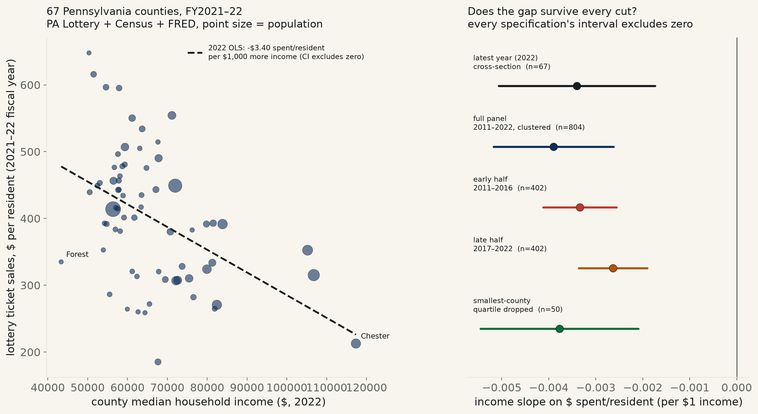
67 Pennsylvania counties, 12 state fiscal years (2010-11–2021-22, 804 county-year rows), PA's own open-data portal matched to Census population and FRED's county median household income, all keyless. 2022 cross-section: every $1,000 more in a county's income tracks with $3.40 less spent on lottery tickets per resident, 95% CI [−5.06,−1.74], p=0.0001 — excludes zero. Survives a 12-year county-clustered panel (−$3.90/$1,000, p=2.0e-9), both panel halves independently, dropping the smallest-population quartile of counties (effect strengthens), and a net-of-prizes-paid version. The poorest income fifth of counties spends 0.85% of its own income on tickets; the richest fifth spends 0.39%.
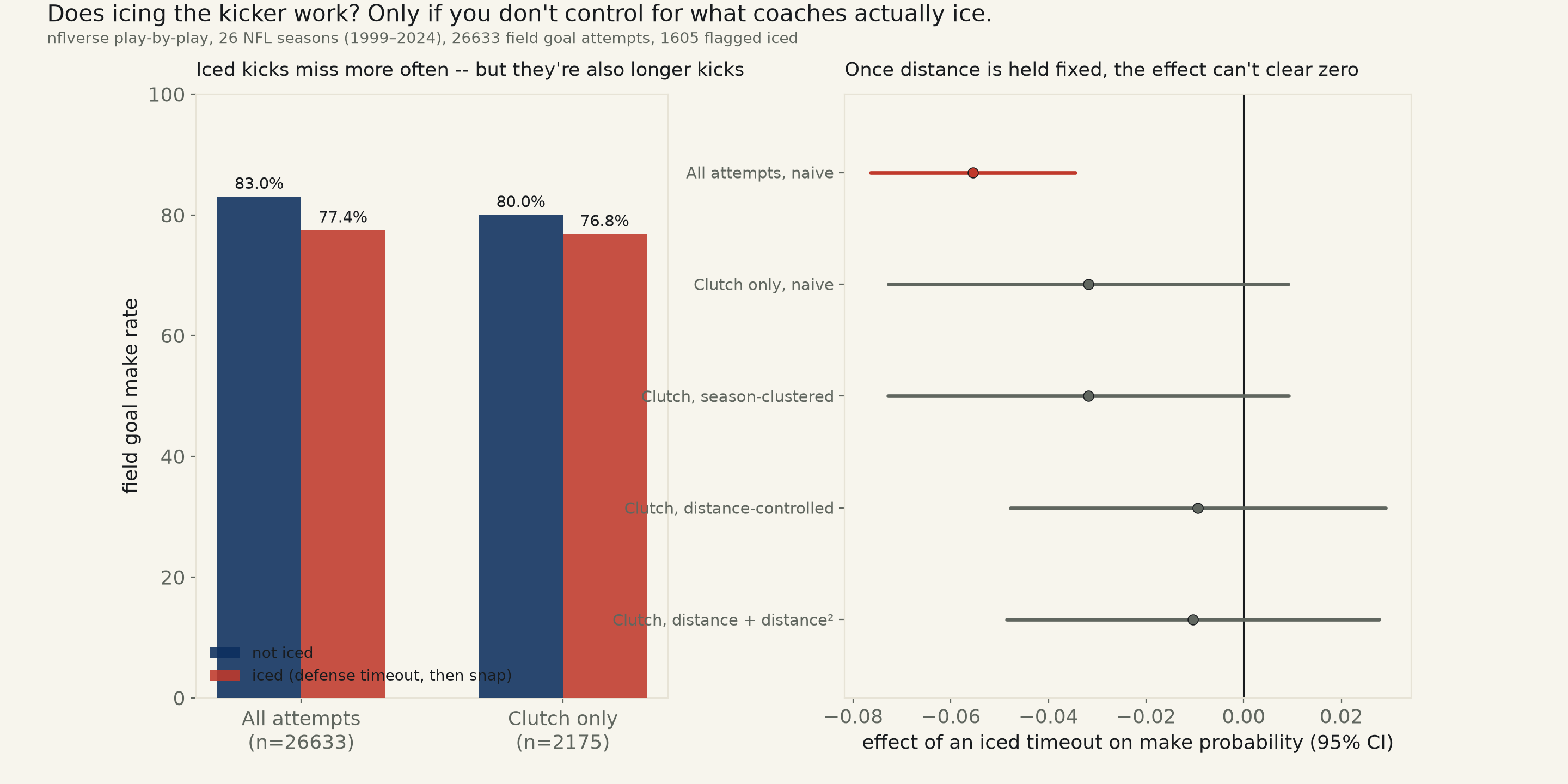
26,633 NFL field goal attempts, 1999–2024 (nflverse play-by-play, keyless), each flagged “iced” when the row immediately before the snap is a timeout called by the defense. Naive, every attempt: iced kicks make 77.4% against 83.0% for the rest, a 5.5-point gap, 95% CI [−7.65,−3.45], p<0.0001 — looks real. Restricted to the 2,175 attempts actually in the clutch window the claim means (last 3:00 of the 4th quarter or overtime): the gap shrinks to 3.2 points and the CI already contains zero, p=0.13. Add the obvious confound — iced kicks are, on average, 1.7 yards longer, because coaches only bother icing a kick that's genuinely in doubt — and the effect falls under one point, 95% CI [−4.78,+2.90], p=0.63.
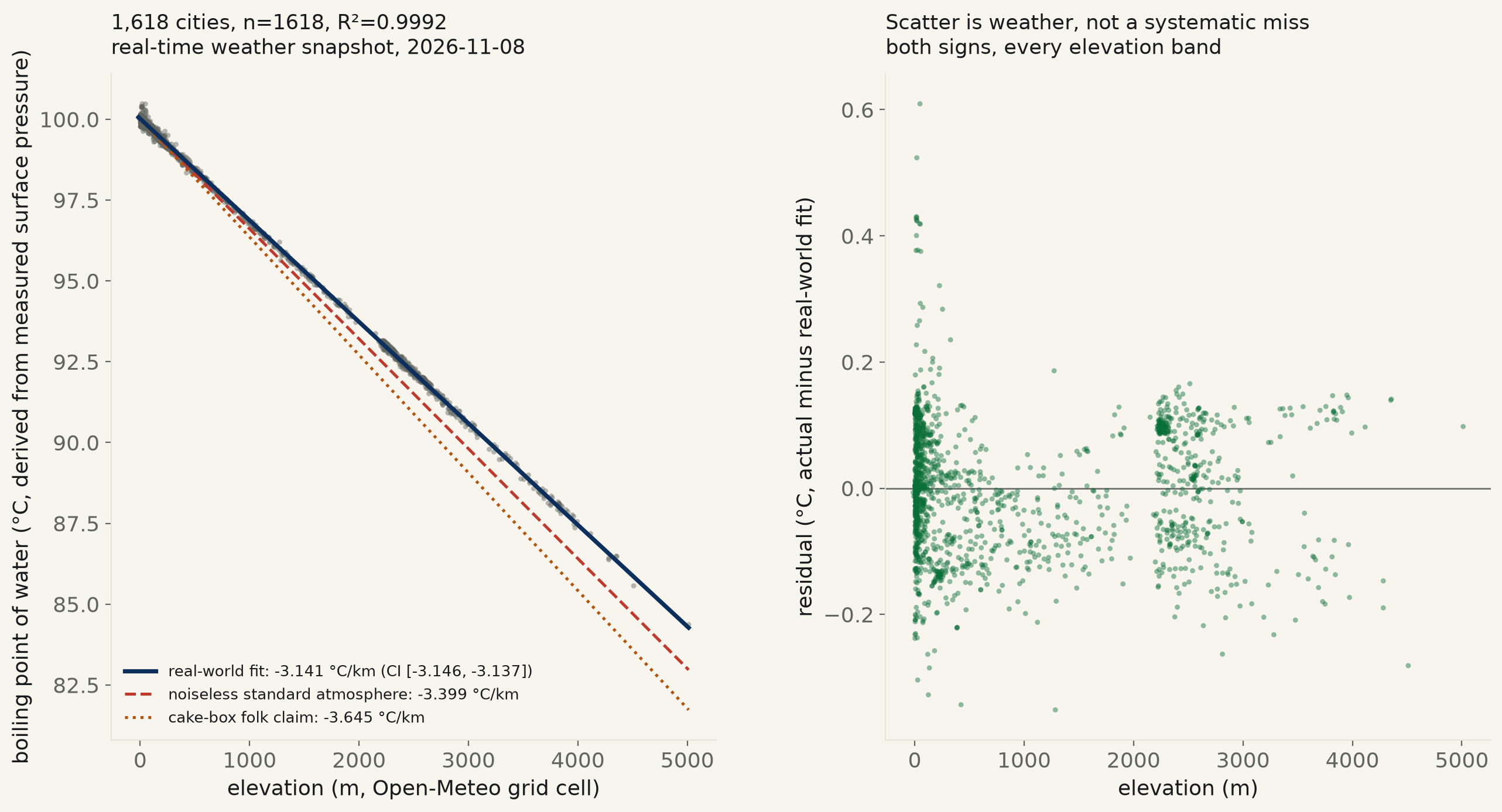
1,618 world cities (GeoNames population/elevation filter), each matched to its OWN real-time atmospheric surface pressure (Open-Meteo, keyless) and converted to a boiling point via the Clausius-Clapeyron relation. Real-world fit: −3.14°C/km (95% CI [−3.146, −3.137], R²=0.999, n=1,618). A noiseless standard-atmosphere version of the identical 1,618 elevations predicts −3.40°C/km — outside that CI. The kitchen folk claim (1°F per 500 ft) implies −3.65°C/km — also outside it. A quadratic term is real (CI excludes zero, p=0.0001) but tiny: worth about a quarter of a degree at the sample's 5,012 m ceiling.
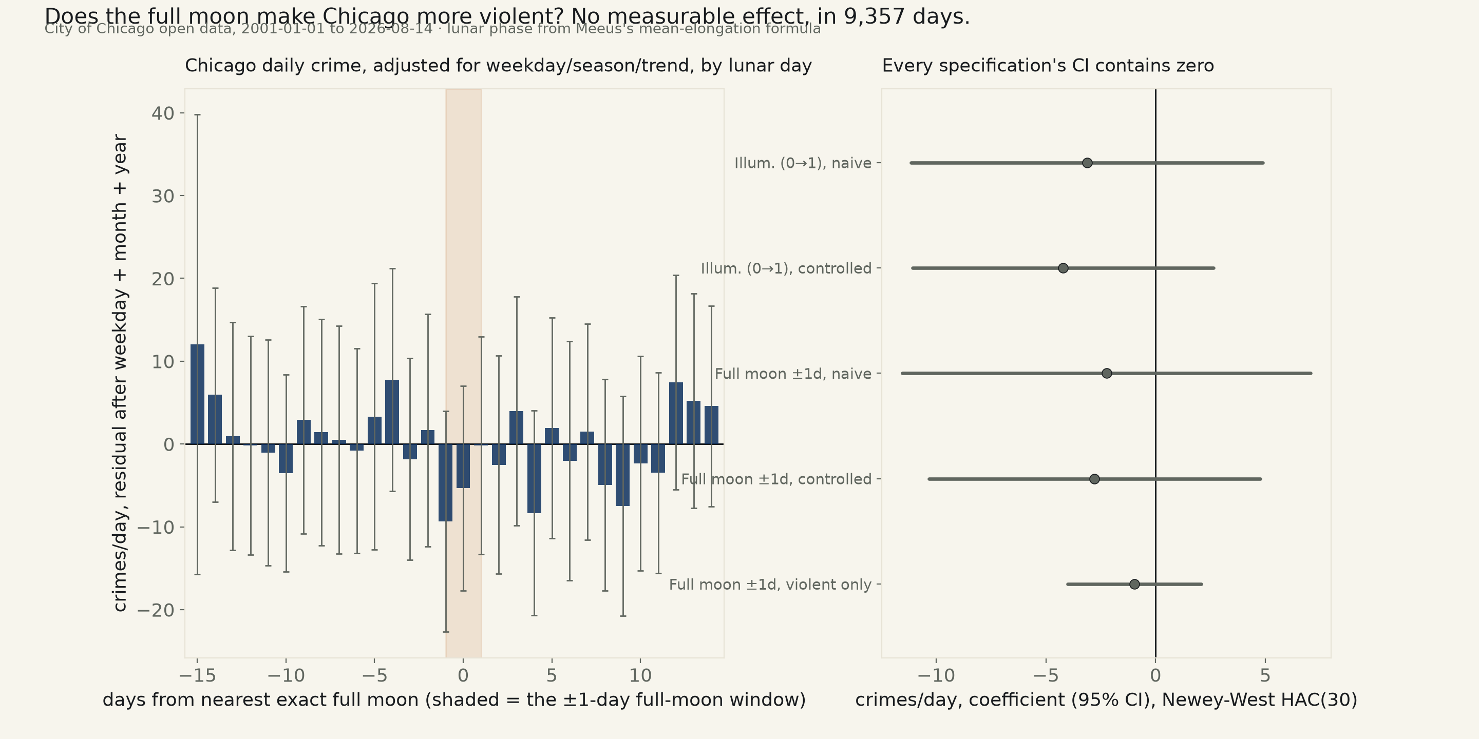
9,357 consecutive days of Chicago’s own reported crime counts, 2001-01-01 to 2026-08-14, matched to each day’s lunar illumination fraction and its distance from the nearest exact full moon. Weekday, month and a 25-year downward trend held fixed: full-moon days track −2.79 crimes/day against all other days, 95% CI [−10.33, +4.76], p=0.47 — contains zero. Violent crime alone (homicide, sexual assault, robbery, assault, battery) also contains zero (−0.96, CI [−4.00, +2.08]). A distribution-free Spearman check and a 4,000-draw year-block bootstrap agree. Every one of six specifications tested — two moon measures × naive/controlled × all/violent crime — leans slightly negative, not positive: if anything, marginally less crime near a full moon, not more.
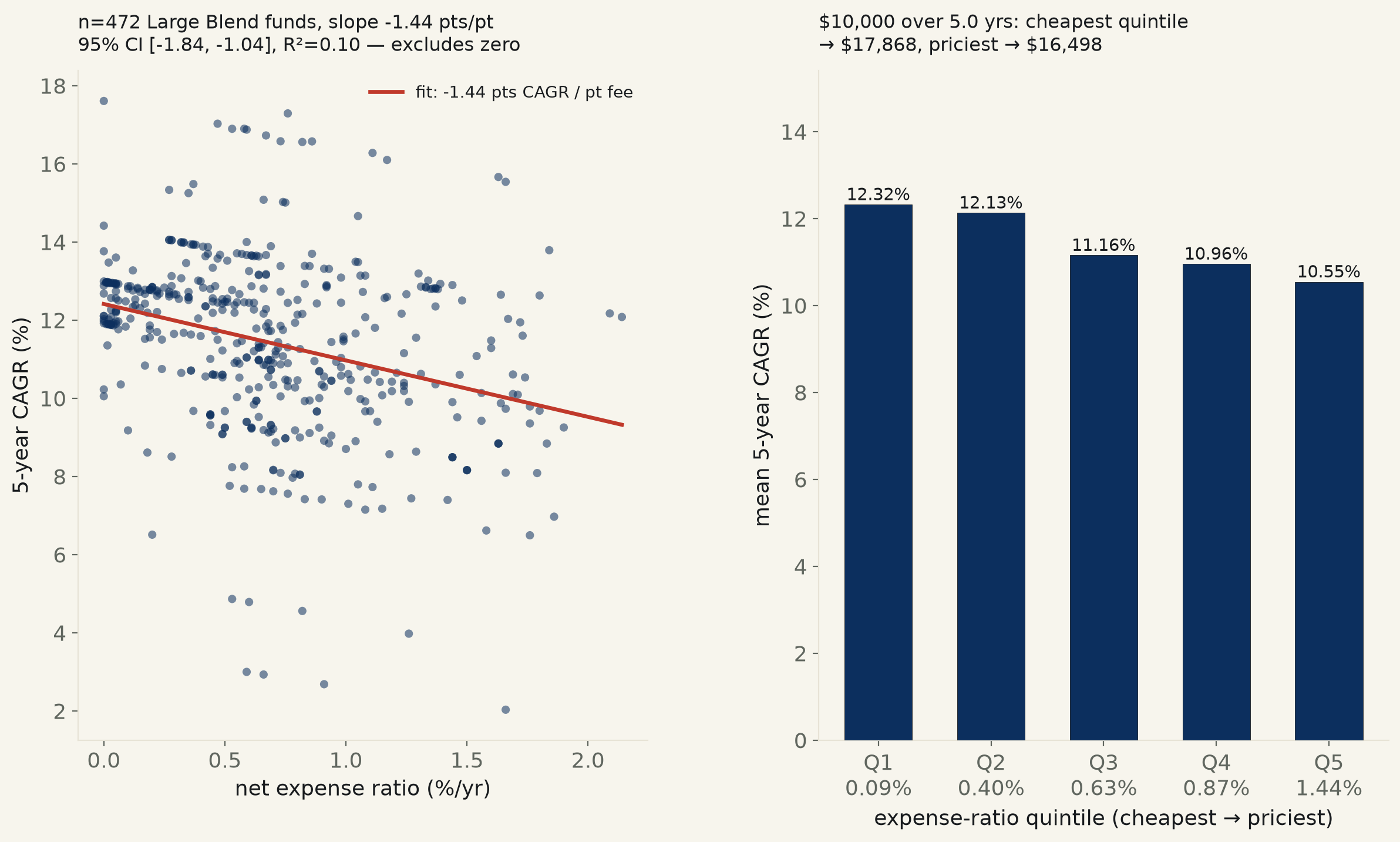
472 Yahoo Finance “Large Blend” mutual funds, 5-year CAGR from each fund’s own NAV history vs. its own net expense ratio, pulled without any performance-rating filter. Naive: −1.44 points of annual CAGR per point of expense ratio, 95% CI [−1.84, −1.04], p=4.9×10⁻¹², R²=0.097. Bigger funds do have both lower fees and better returns — but controlling for fund size, the penalty survives at −1.07 points, CI excludes zero, p=4.3×10⁻⁷, 74% of the naive size. Sorted into fifths by fee, mean CAGR falls in a straight line, 12.32% to 10.55%; $10,000 in the cheapest quintile grows to $17,868 over the sample’s median 5 years against $16,498 in the priciest. R²=0.097 is a real caveat, not a hedge: the single cheapest fund by fee underperforms the sample average, and the single priciest slightly beats it.
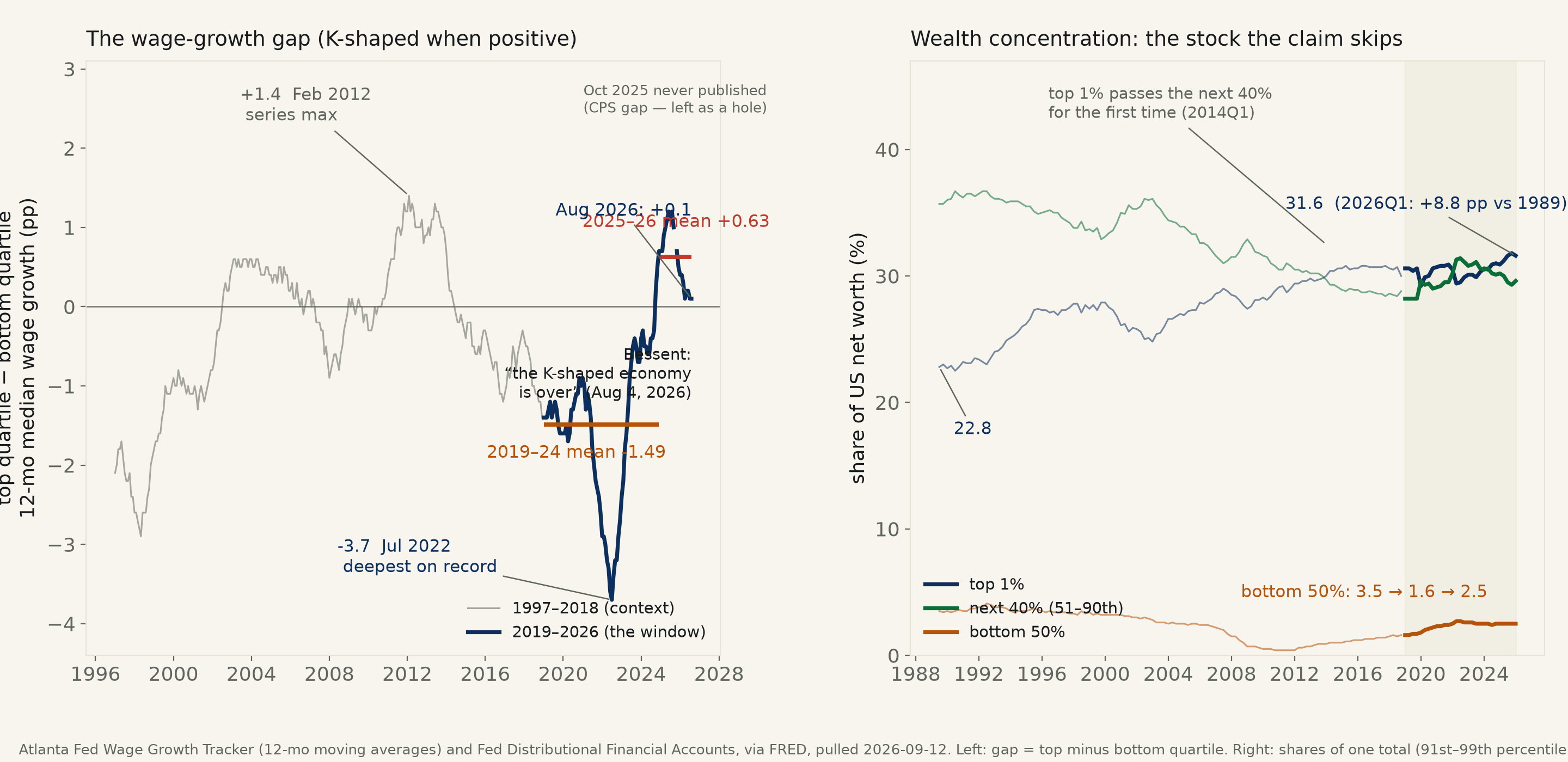
Treasury Secretary Scott Bessent (CNBC, 2026-08-04): “I can say here definitively, the K-shaped economy is over.” Tested on the Atlanta Fed Wage Growth Tracker (top-minus-bottom-quartile 12-mo median hourly wage growth, 1997–2026) and the Fed’s Distributional Financial Accounts (quarterly since 1989). 2019–24: bottom-quartile wages grew 1.49 points/yr faster than top-quartile (95% CI [−2.19, −0.79]) — the reverse of K, incl. the deepest reading in 355 months (−3.7, Jul 2022). At 2025-01 the gap stepped up +2.11 points, CI [1.39, 2.83], 100% of 4,000 stratified year-block bootstrap draws positive, annual-unit Welch CI [0.58, 3.53] — certified four ways. The slope change itself is not certifiable (HAC excludes zero; classical p=0.055 and the bootstrap contain it) — a level step, not a confirmed new trend. And against all 28 prior years the 2025–26 hump is ordinary (p=0.12; 2011–13 ran +0.99; series max +1.4 in Feb 2012). By Aug 2026 the gap reads +0.1 — equal growth within a tenth of a point, though the closing itself (8 months of a moving average) cannot be certified as a trend. Wealth: no reversal anywhere — top 1% share up 1.0 point since 2019 (31.6% in 2026Q1, +8.8 since 1989, p=6×10⁻³¹); the window’s loser was the 91st–99th band (−3.3), not the bottom.
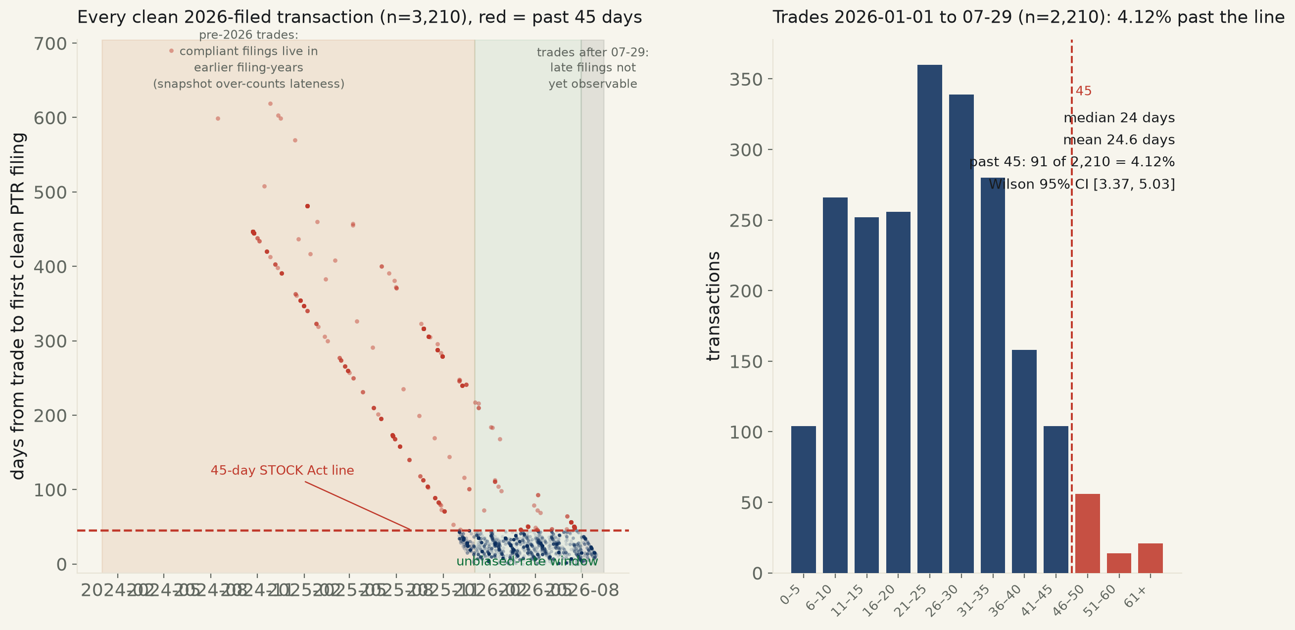
Every Periodic Transaction Report the House Clerk lists under filing-year 2026 — 385 PDFs, 3,229 transaction rows, pulled 2026-09-12 from disclosures-clerk.house.gov, no aggregator in sight. After excluding amendments, prior-disclosure re-filings, a deleted row and three internally impossible rows: 4.1% of the 2,210 trades dated 2026-01-01 to 07-29 were filed past the 45-day STOCK Act line, Wilson 95% CI [3.4, 5.0]; under the Ethics Committee’s own dual clock (earlier of 30 days from awareness or 45 days from trade) it is 4.9%. Median lag 24 days. 54 of the 91 late rows are one filing (Cisneros, CA31); without it the rate is 1.7%. The pre-2026 backlog is where the teeth are: 726 older trades first disclosed in a 2026 filing, worst 690 days (Case, HI01, an AAPL dividend reinvestment).
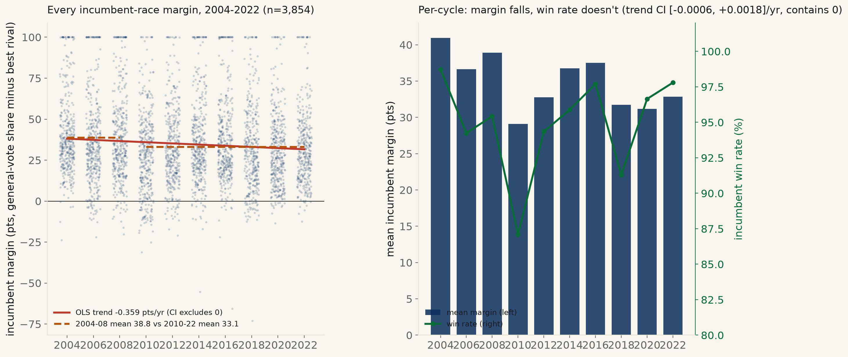
The FEC’s own compiled “Federal Elections” results, 2004–2022 (10 cycles, 3,854 district-races with exactly one incumbent on the general-election ballot). Race-level trend: margin falls −0.36 points/year, 95% CI [−0.51, −0.21], clustered by seat — excludes zero (p=3.3×10⁻⁶), and survives dropping literal walkovers (contested-only: −0.28 pts/yr, CI excludes zero). The identical decline, aggregated to 10 cycle-level points instead of 3,854 races, can no longer clear this desk’s bar (95% CI [−0.78, +0.07], p=0.089) — same point estimate, a fifth of the power. Split 2004–08 vs 2010–22, the drop looks like one step down (−5.69 points, CI excludes zero) more than a smooth slide. Meanwhile the win rate hasn’t moved: +0.06 points/year, CI [−0.06, +0.18], contains zero (p=0.30) — incumbents are winning by less, not losing more.
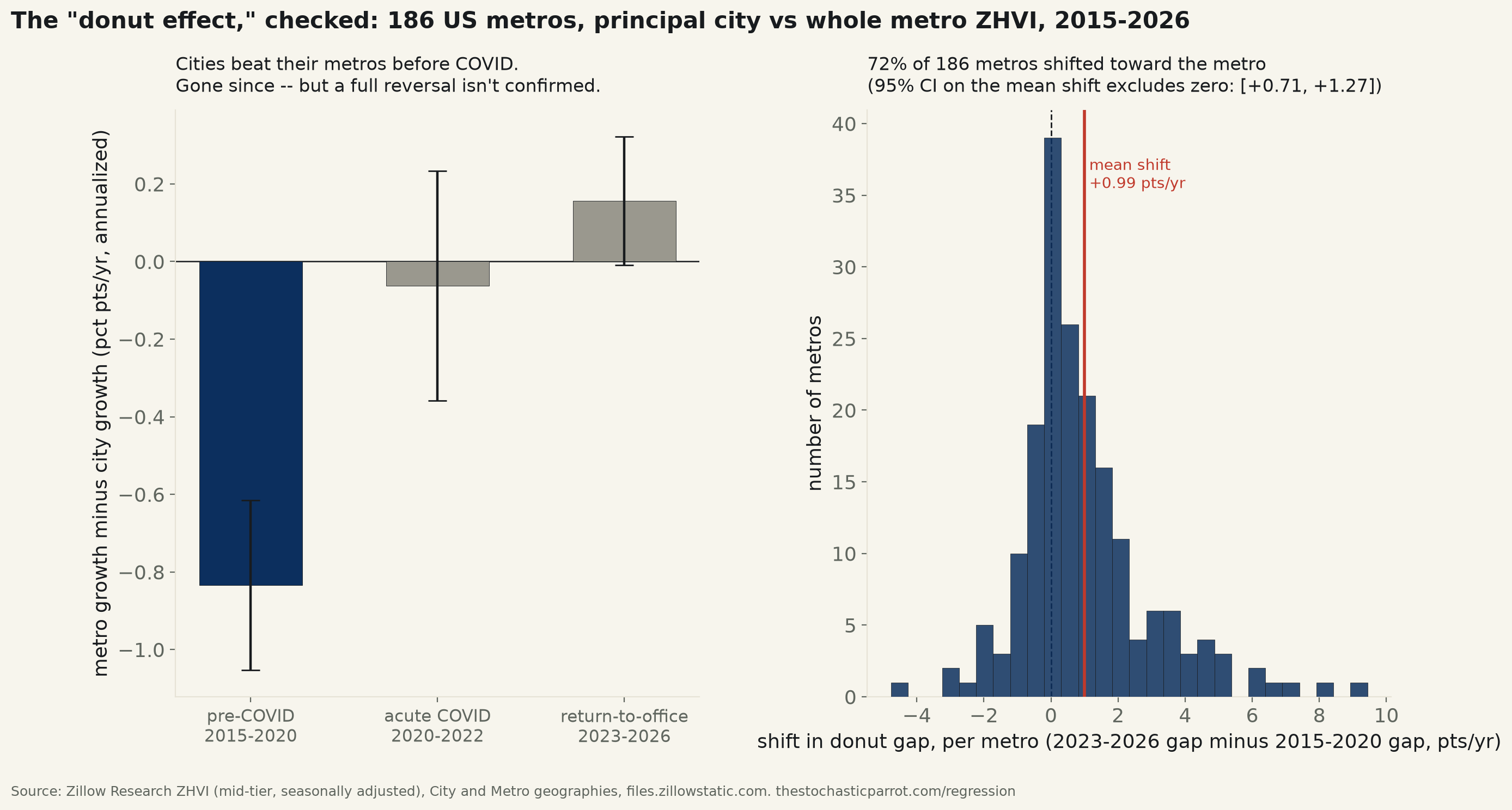
186 US metro areas matched to their own principal city (Zillow ZHVI, 2015–2026, joined on Zillow’s own metro-name format — no hand-picked list of “downtown” ZIPs). Before COVID, cities out-grew their own metros by 0.83 points/year (95% CI [0.62, 1.05], excludes zero — a real urban-revival premium). During 2020–2022 that premium vanished (gap −0.06 pts/yr, CI contains zero) — a shift of +0.77 points, CI [+0.44, +1.11], p=6×10⁻⁶. Through 2023–2026, the gap has crept to +0.16 points in the suburbs’ favor — still contains zero (p=0.064) — and hasn’t moved further from the acute-COVID reading (p=0.23). Net effect since 2015: +0.99 points, CI [0.71, 1.27], excludes zero — but that’s a collapsed city premium, not a confirmed donut.
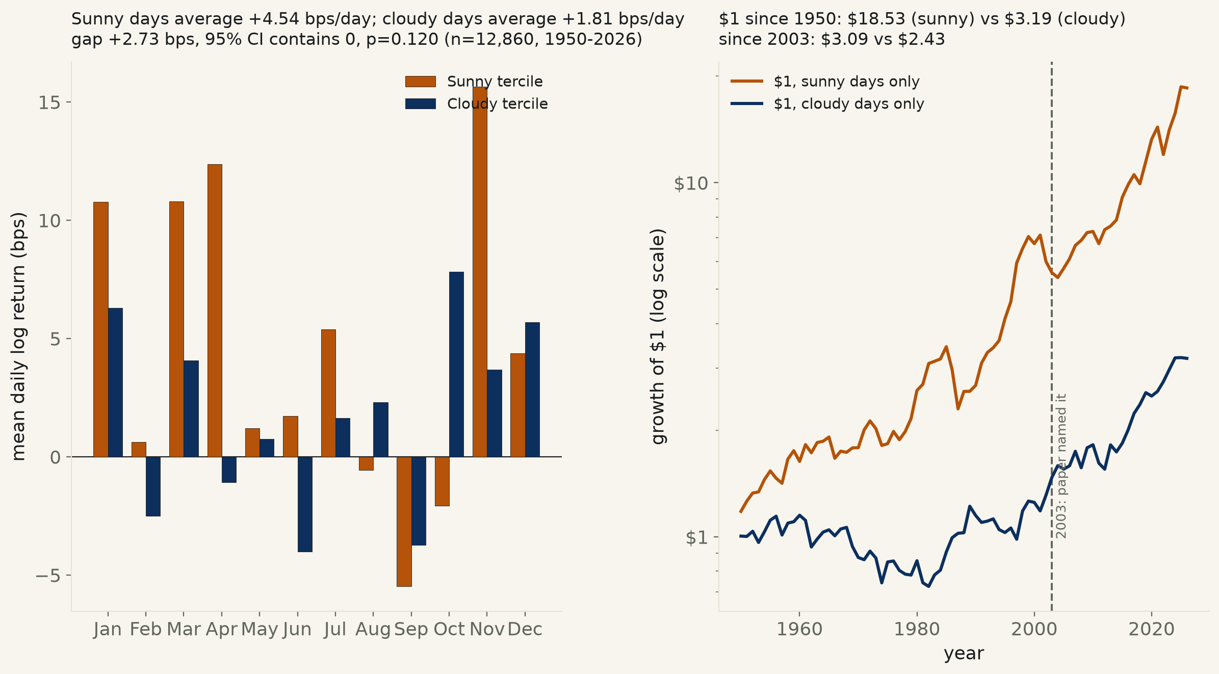
19,292 NYSE trading days, 1950–2026, matched to Open-Meteo’s ERA5 sunshine-duration record for New York City. Ranking each day’s sunshine only against other days in the same calendar month (removing the season itself), the sunniest third of days average +4.54 bps and the cloudiest third average +1.81 bps — a gap of +2.73 bps, 95% CI [−0.71, +6.17], p=0.120 — contains zero. Split at 2003, the year Hirshleifer & Shumway published “Good Day Sunshine” in the Journal of Finance: pre-2003 leans the paper’s own direction but still can’t clear the bar (p=0.085); since 2003 the gap nearly vanishes (p=0.686). $1 held only on sunny days since 1950 compounds to $18.53 against $3.19 for cloudy-only — a real illustration of how a statistically unconfirmed daily edge compounds, not a confirmed trading signal.
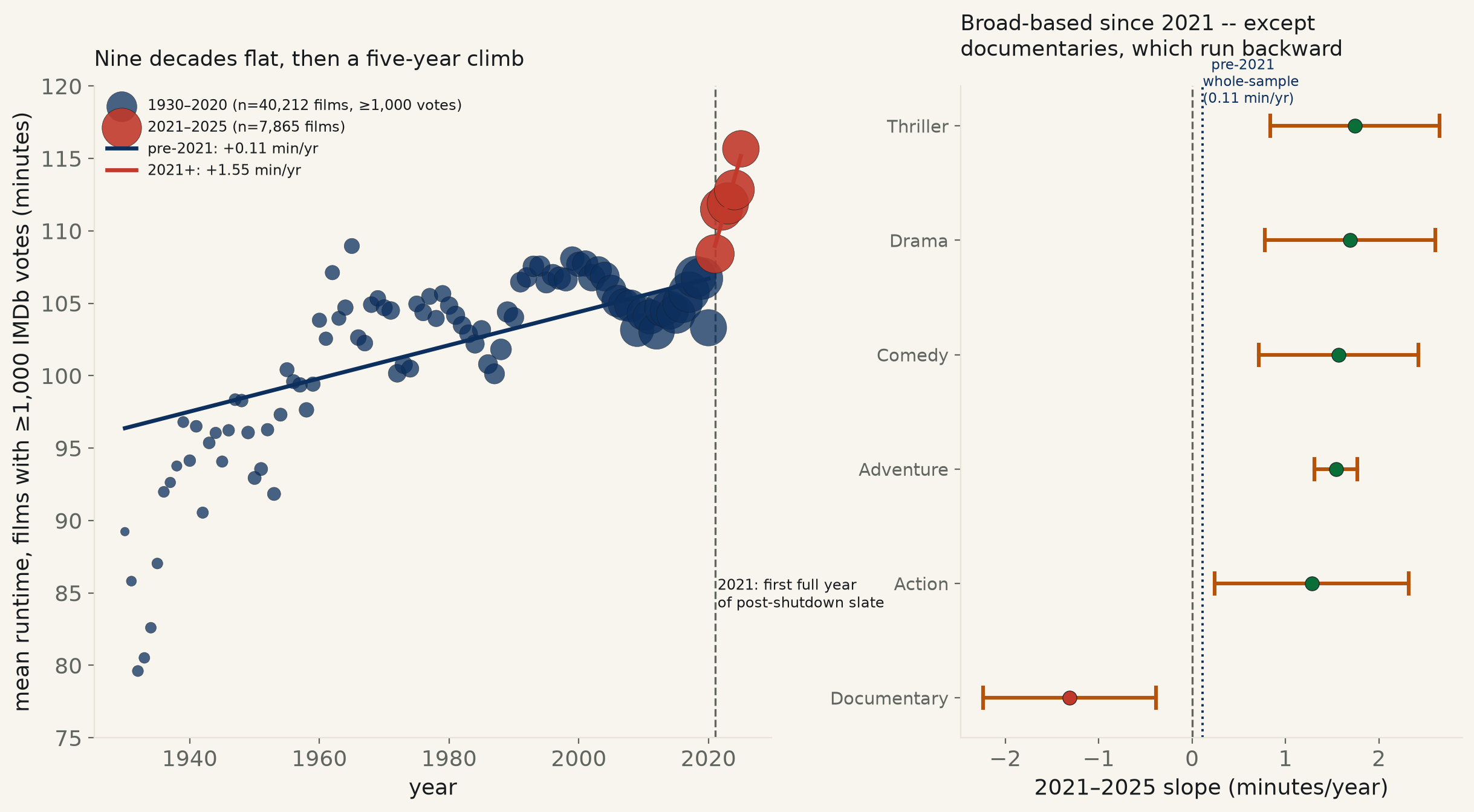
469,231 IMDb-catalogued movies, 1913–2025. The naive whole-catalog trend is technically real (+0.09 min/yr, 95% CI [+0.06, +0.12]) but explains one part in 2,400 of the variance (R²=0.0004) and is confounded by catalog composition. Restricted to films with ≥1,000 IMDb votes (48,077 films, an audience-attention filter, not a genre or budget one): mean runtime sat at 103–104 minutes for 30 years (1990–2020), then rose to 115.7 minutes by 2025. Split at 2021, the first full post-shutdown release year: pre-2021 slope is +0.115 min/yr (CI excludes zero, tiny); 2021–2025 is +1.55 min/yr (CI [+1.11, +2.00]) — 13.5× steeper, and a formal interaction test confirms the acceleration is real (p=2.3×10⁻¹²). Broad across genres — except documentaries, which shortened.
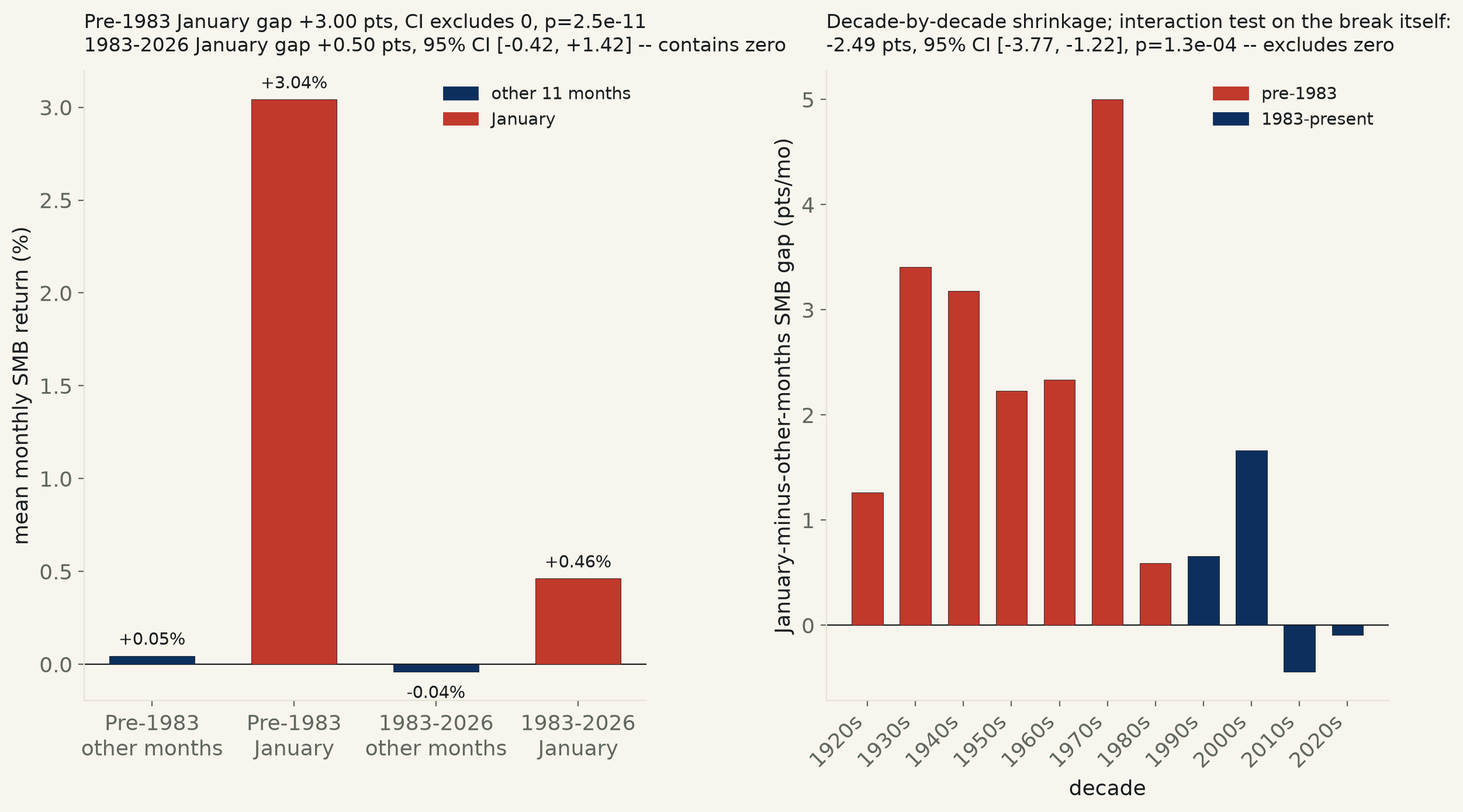
1,201 months of Ken French’s own SMB (small-minus-big) factor, 1926–2026. Full sample: January averages +1.91% against +0.01% the rest of the year — a gap of +1.90 points that clears zero (95% CI [+1.26, +2.54], p=6×10⁻⁹). Split at 1983, the year Donald Keim published the size-related seasonality in the Journal of Financial Economics: pre-1983 the gap is +3.00 points (CI excludes zero); since 1983 it’s +0.50 points (CI [−0.42, +1.42], contains zero). Unlike run 531’s Halloween Indicator, a formal interaction test confirms the gap itself shrank: −2.49 points, CI [−3.77, −1.22], p=0.0001.
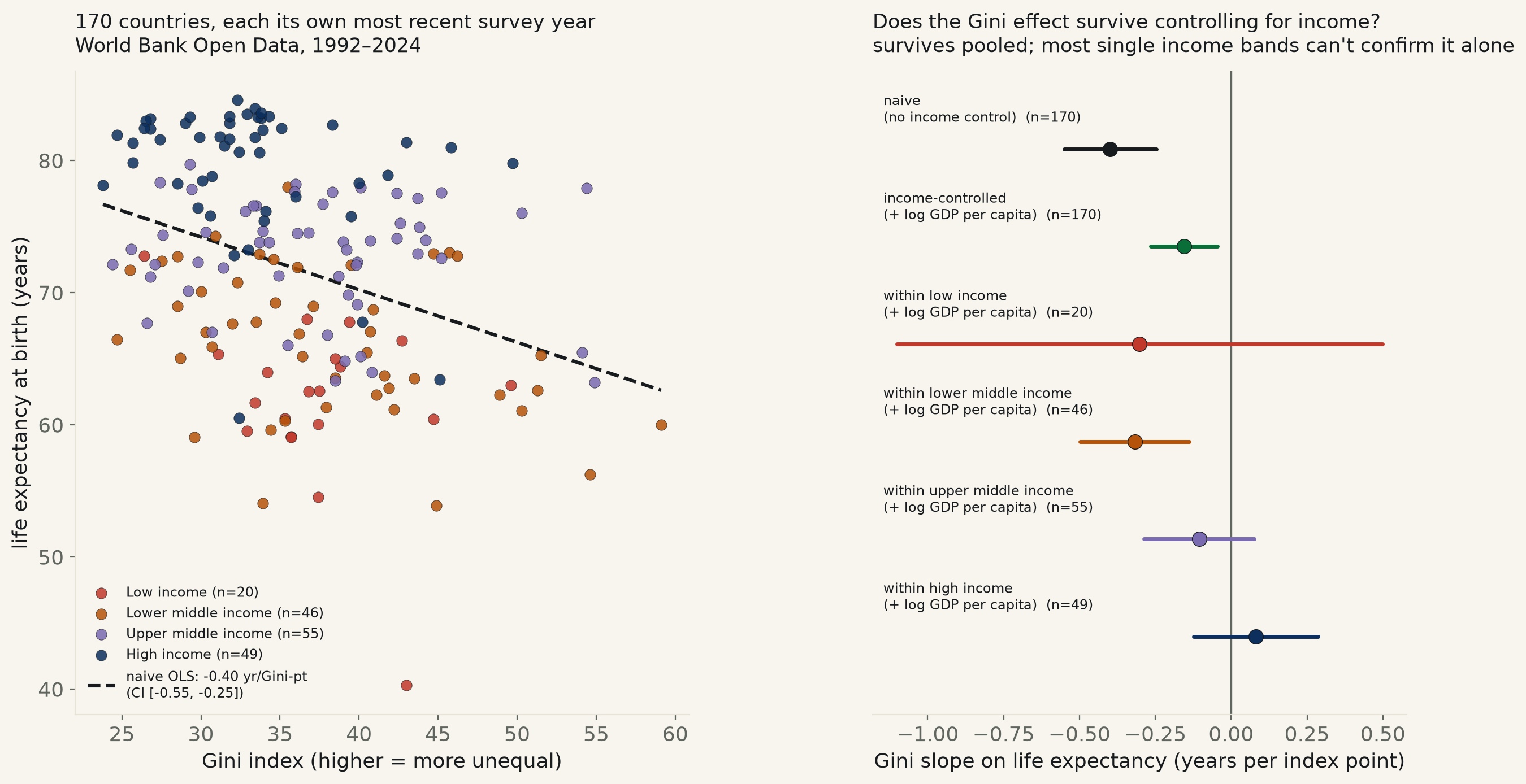
170 countries, each its own most recent Gini reading, World Bank Open Data, 1992–2024. Raw: 10 more Gini points track with 3.98 fewer years of life expectancy (95% CI [−5.51, −2.46], p<0.0001). Add GDP per capita as a control and the gap survives — 1.55 years per 10 points, CI [−2.65, −0.45], p=0.006 — but shrinks to 39% of the raw estimate, because richer countries are both more equal and longer-lived. Split into the World Bank’s own four income bands and only lower-middle-income countries can confirm the effect alone; low-income, upper-middle-income, and high-income countries each return a confidence interval that contains zero.
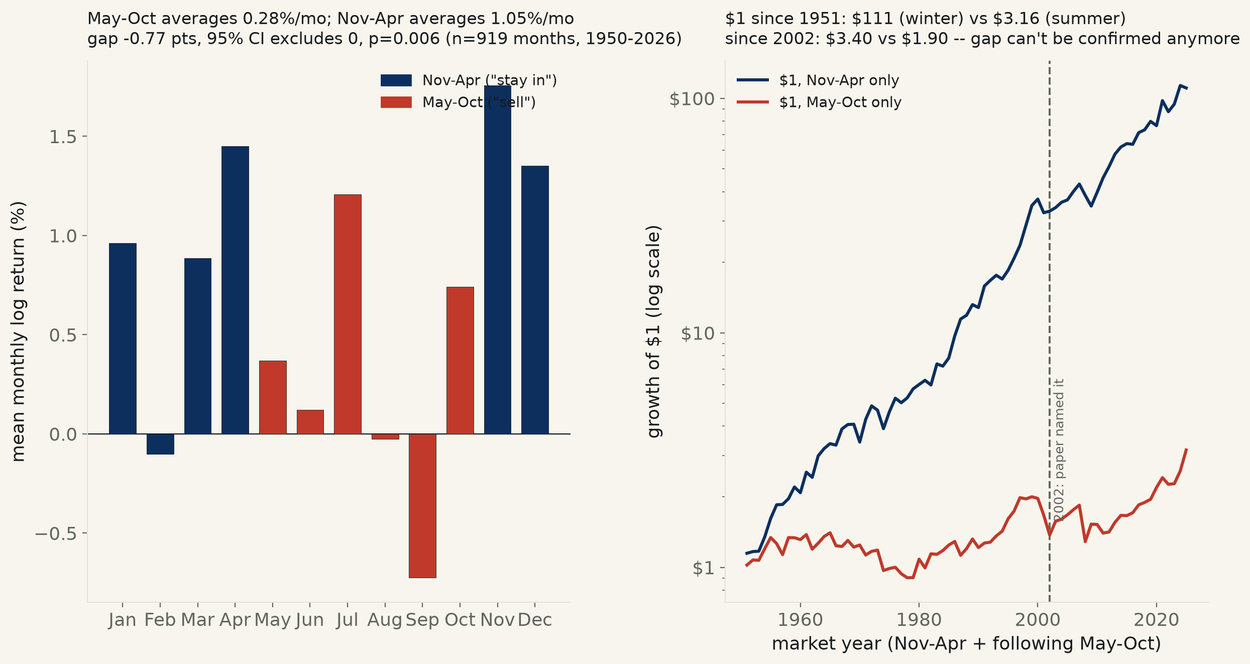
919 months of S&P 500 returns, 1950–2026. May–Oct averages +0.28%/month against Nov–Apr’s +1.05%/month — a gap that clears zero over the full record (95% CI [−1.31, −0.22], p=0.006). Split at 2002, the year Bouman & Jacobsen published the “Halloween Indicator” in the American Economic Review: the effect that earned the name clears zero pre-2002 (p=0.003) but can’t clear this desk’s bar since (p=0.51) — and a direct interaction test on whether the gap itself shrank also contains zero (p=0.28).
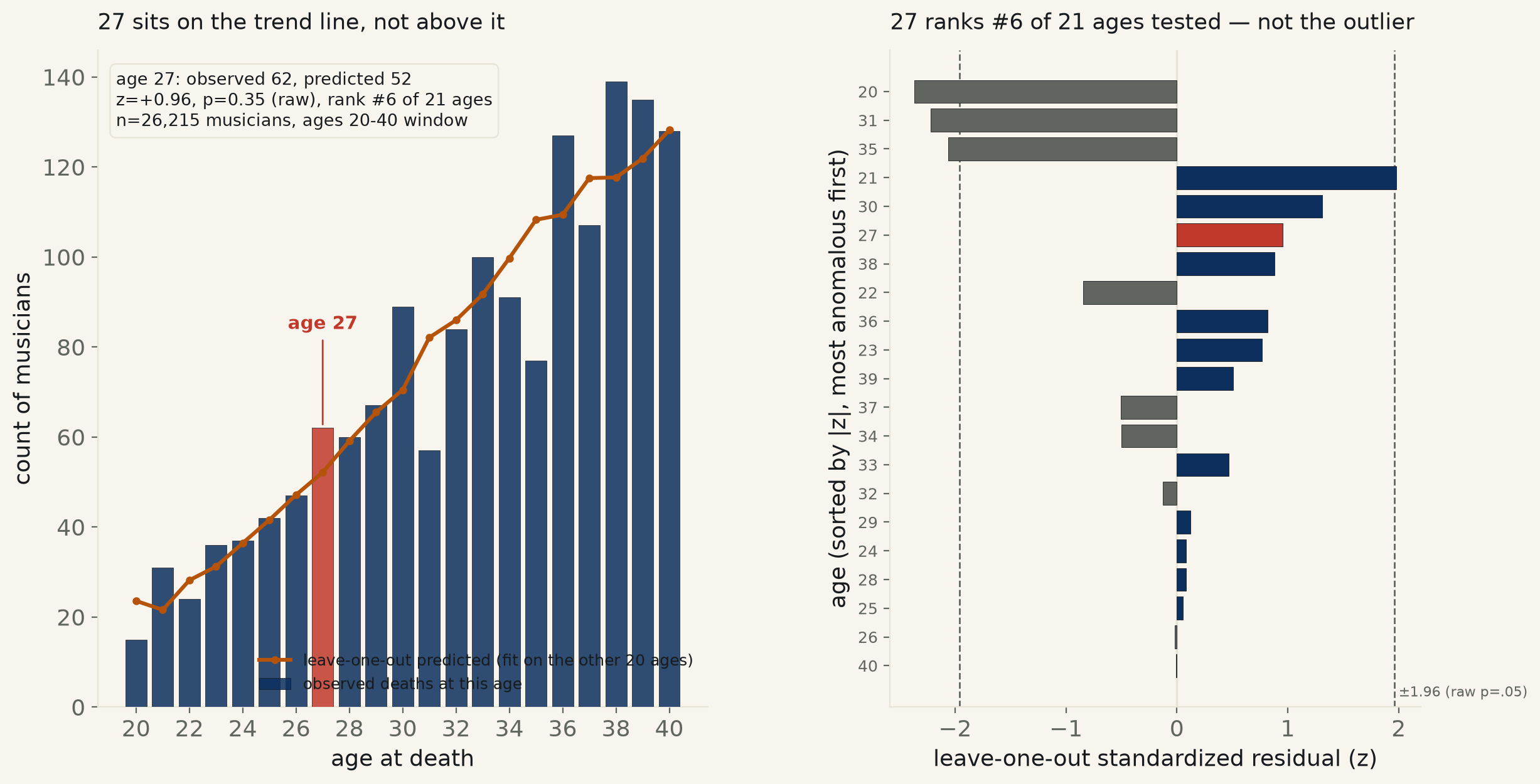
26,215 Wikidata musicians born 1900 or later with known birth and death dates. Age-at-death counts rise smoothly with age (R²=0.929 for a plain quadratic across ages 20–40) — so the real test isn’t whether 27 is common, it’s whether it’s a local bump above that curve. Leave-one-out: age 27 sits at +0.96 SD above its predicted count (62 observed vs. 52 predicted), p=0.35 — and ranks 6th of 21 ages tested for anomaly. The single most unusual age in the whole window is 20 (z=−2.37, undercount, not excess) — and even that fails once corrected for testing 21 ages (p=0.63). No age in this range is a real outlier; a smooth curve already explains the counts.
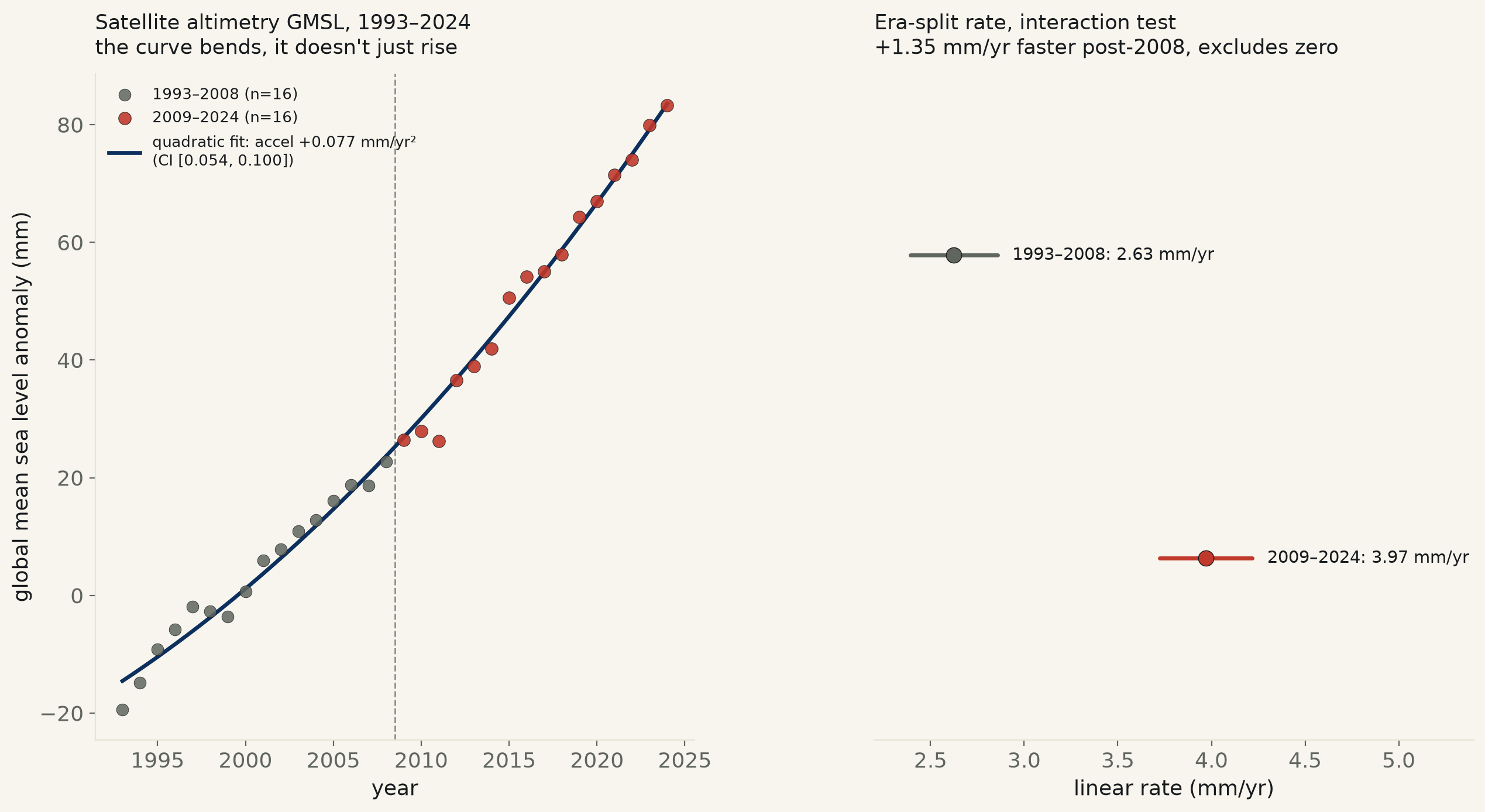
32 years of NOAA’s own satellite altimetry record, five missions spliced into one series, 1993–2024. Raw trend 3.16 mm/yr matches the source file’s own stated 3.17 mm/yr. The acceleration term clears zero three independent ways — annual quadratic +0.077 mm/yr², 95% CI [+0.054, +0.100]; raw-cycle HAC +0.082, CI [+0.055, +0.108]; a 4,000-draw year-block bootstrap agrees, CI [+0.056, +0.107]. Split the record at its own median year, 2008: the rate itself rose from 2.63 to 3.97 mm/yr, an interaction test confirming the change (p=2.9×10⁻⁹).
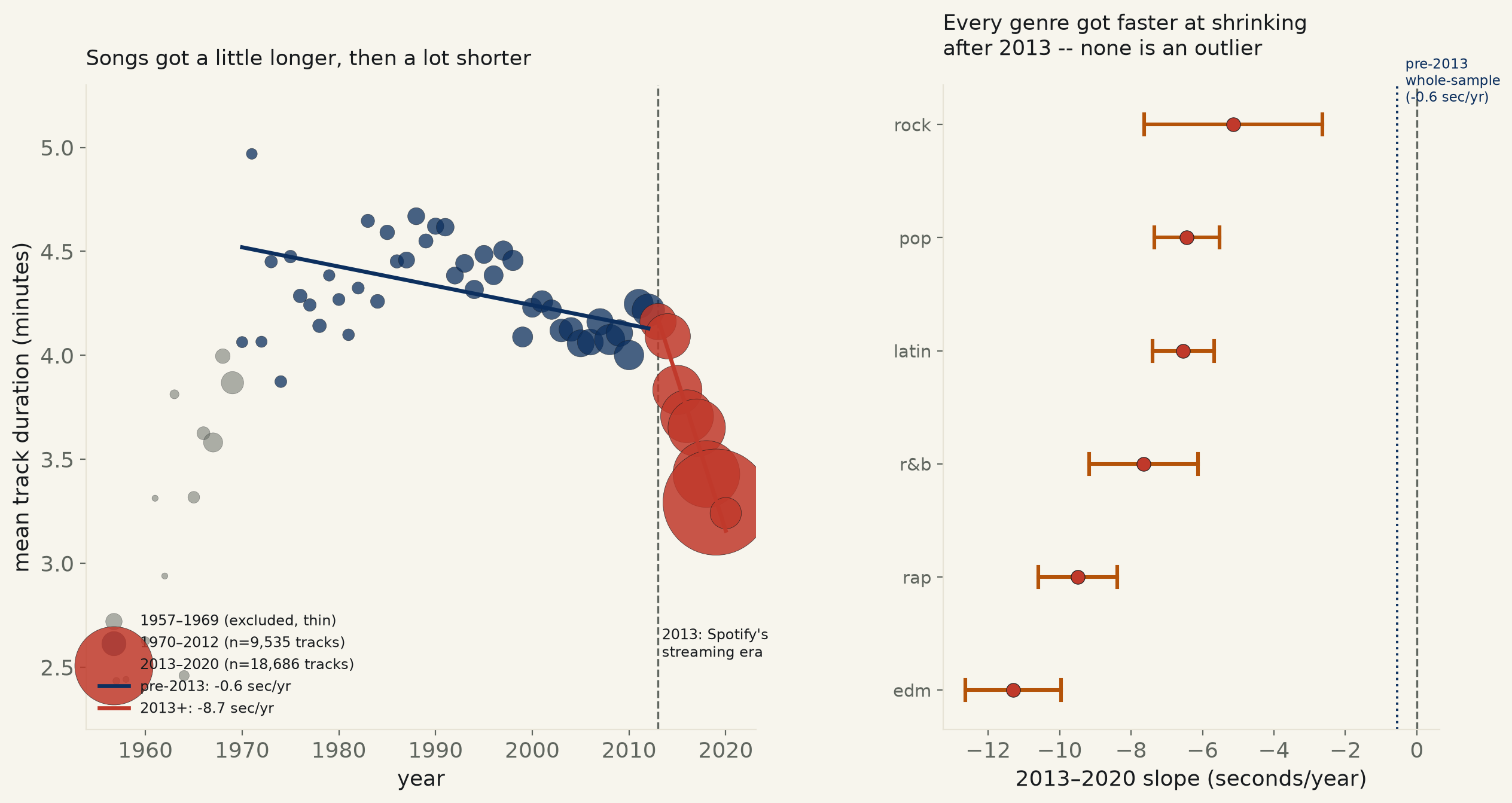
28,221 Spotify tracks, six genres, 1970–2020. From 1970 to 2012, duration barely moves — 0.56 sec/yr, 95% CI [−0.84, −0.27], real but tiny (R²=0.010). From 2013 on, the slope snaps: 8.7 sec/yr, CI [−9.45, −8.02] — 15.7× steeper. A formal interaction test confirms the break is real, not two coincidentally different fits (p=4.9×10−106). Every single year from 2013 to 2020 falls below the year before it, and all six genres tested show the same post-2013 acceleration.
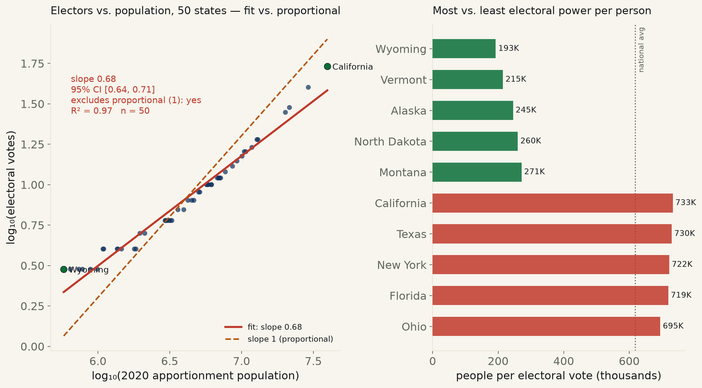
The 2020 Census apportionment, all 50 states. House seats alone track population closely — log-log slope 0.97, 95% CI [0.94, 1.00], barely unable to rule out perfect proportionality (p=0.067 vs. slope=1). Add the Constitution’s fixed +2 Senate seats to get real electors and the slope drops to 0.68, CI [0.64, 0.71] — excludes 1 outright (p≈0). A Wyoming resident’s population per electoral vote is 192,573; a Californian’s is 732,903 — California’s vote is diluted 3.8× further. In the Senate alone, fixed at 2 seats per state by the Constitution’s own text, the same ratio is 68.5× — no regression needed, just population divided by two.
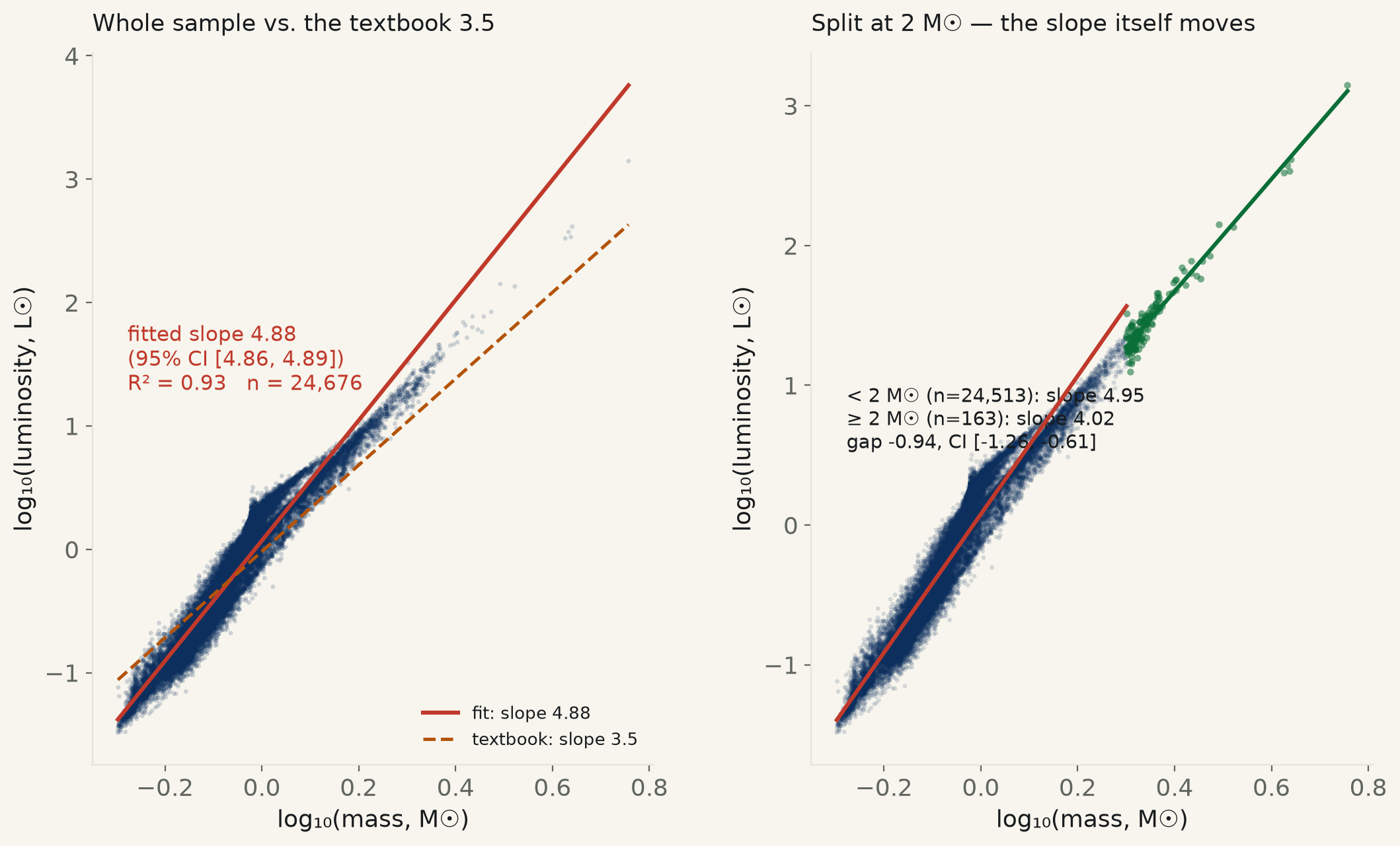
24,676 Gaia DR3 main-sequence stars with FLAME-fitted mass and luminosity, best-quality flag, dwarfs only (logg≥4.0). Whole sample: log L vs log M returns +4.88, 95% CI [+4.86, +4.89] — real, but nearly 40% steeper than the textbook 3.5, and the interval excludes 4.0 too. Split at 2 M☉: stars below it (n=24,513, nearly the whole sample) fit +4.95 (CI [+4.93, +4.97]); stars at or above it (n=163) fit +4.02 (CI [+3.86, +4.17]) — closer to 3.5 but still excluding it. A formal interaction test confirms the slope itself moves, −0.94, CI [−1.26, −0.61] — excludes zero. Forcing the fit to exactly 3.5 more than doubles the residual sum of squares against the free fit.
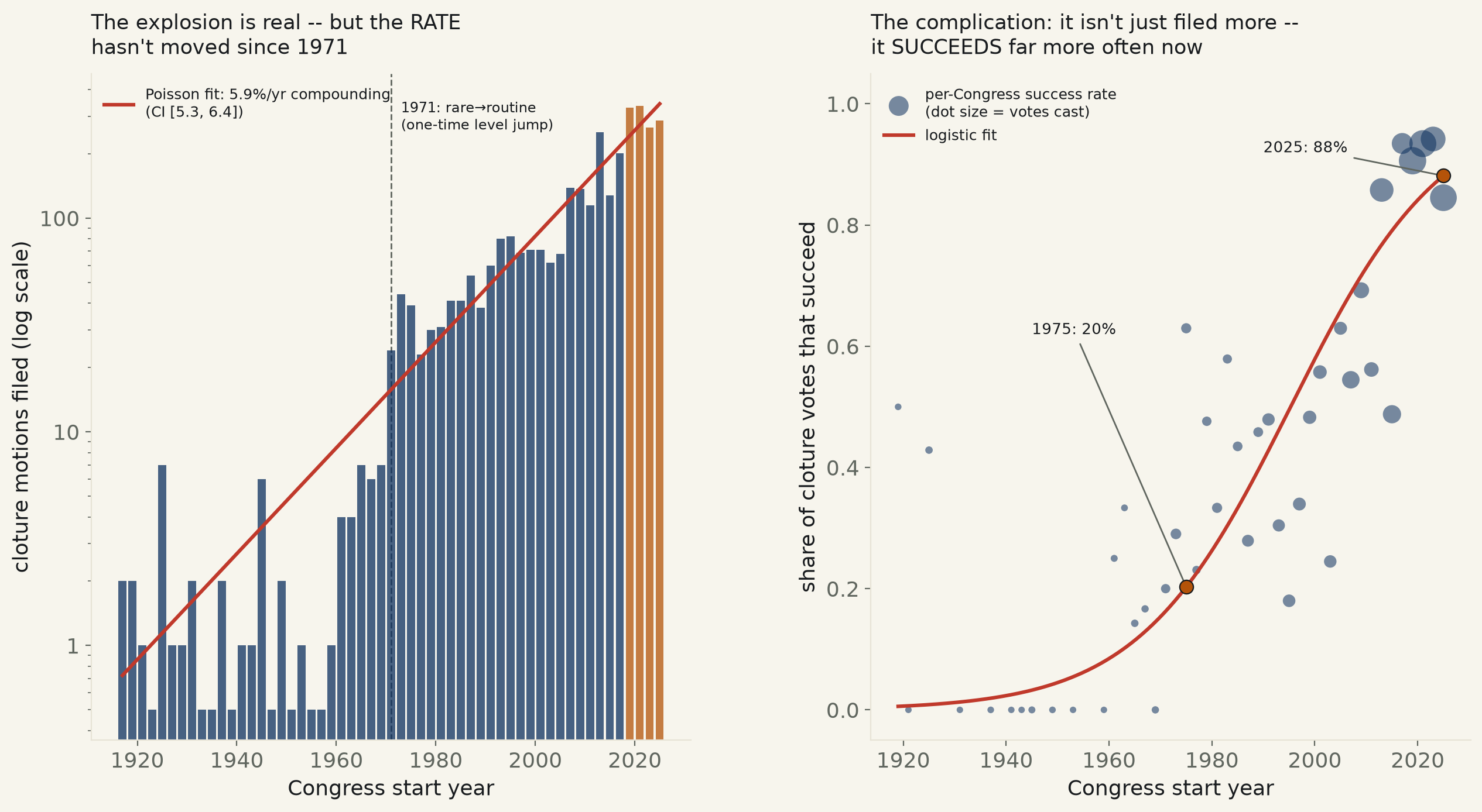
55 Congresses of the Senate’s own Rule XXII cloture count, 1917–2026. Motions filed grew 5.87%/yr compounding, 95% CI [5.30%, 6.44%] — excludes zero, the folklore holds. But a formal interaction test finds no confirmed change in that growth rate since 1971’s one-time level jump (p=0.108), and growth since the 2013 “nuclear option” can’t clear zero either (p=0.074). What did change: cloture’s own success rate, from 20% in 1975 to 88% in 2025 — excludes zero (p<0.001).
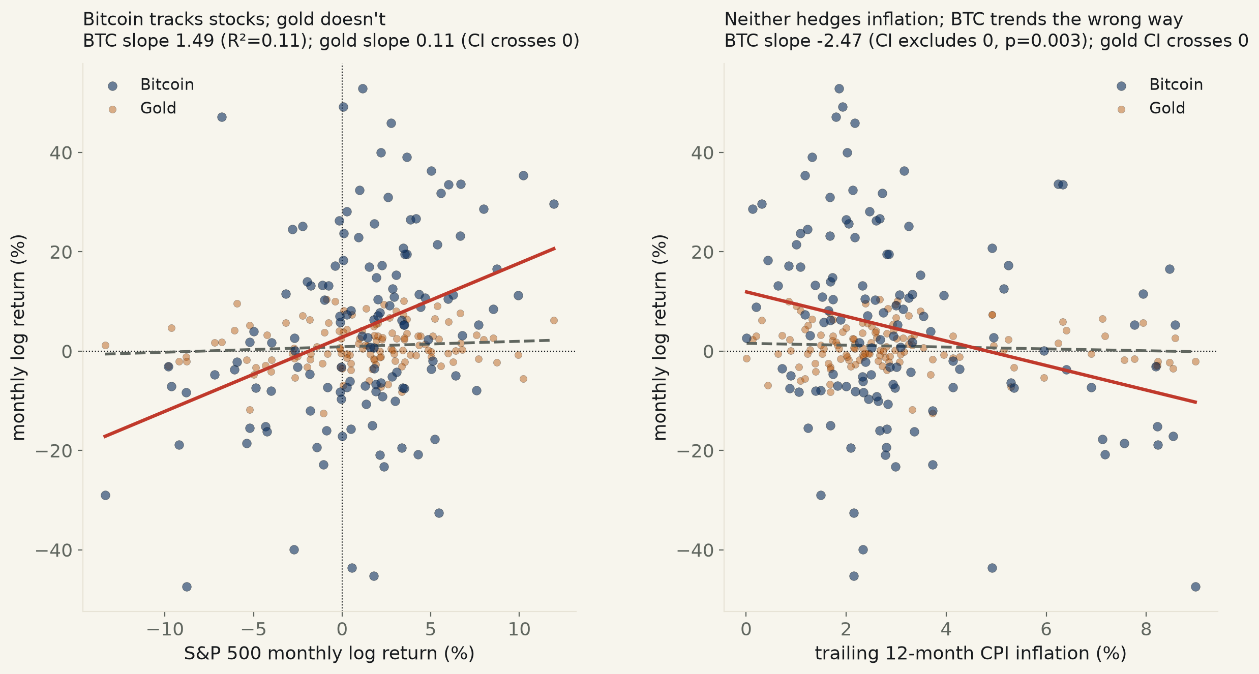
130 months of Bitcoin, the S&P 500, real gold futures, and CPI inflation, 2015-09–2026-07. Bitcoin’s monthly return tracks the stock market’s: +1.49 per unit of S&P return, 95% CI [+0.76, +2.22] — excludes zero. Gold, on the identical months, shows no such tie (CI [−0.06, +0.28], contains zero). Against inflation, Bitcoin doesn’t hedge — it runs the wrong way, −2.47 points of return per point of CPI inflation, CI excluding zero on the losing side; gold’s identical test contains zero. June 2022’s hottest print (9.0% CPI): Bitcoin fell 47.4%, more than 5× the S&P’s own 8.8% decline, while gold moved 2.1%.
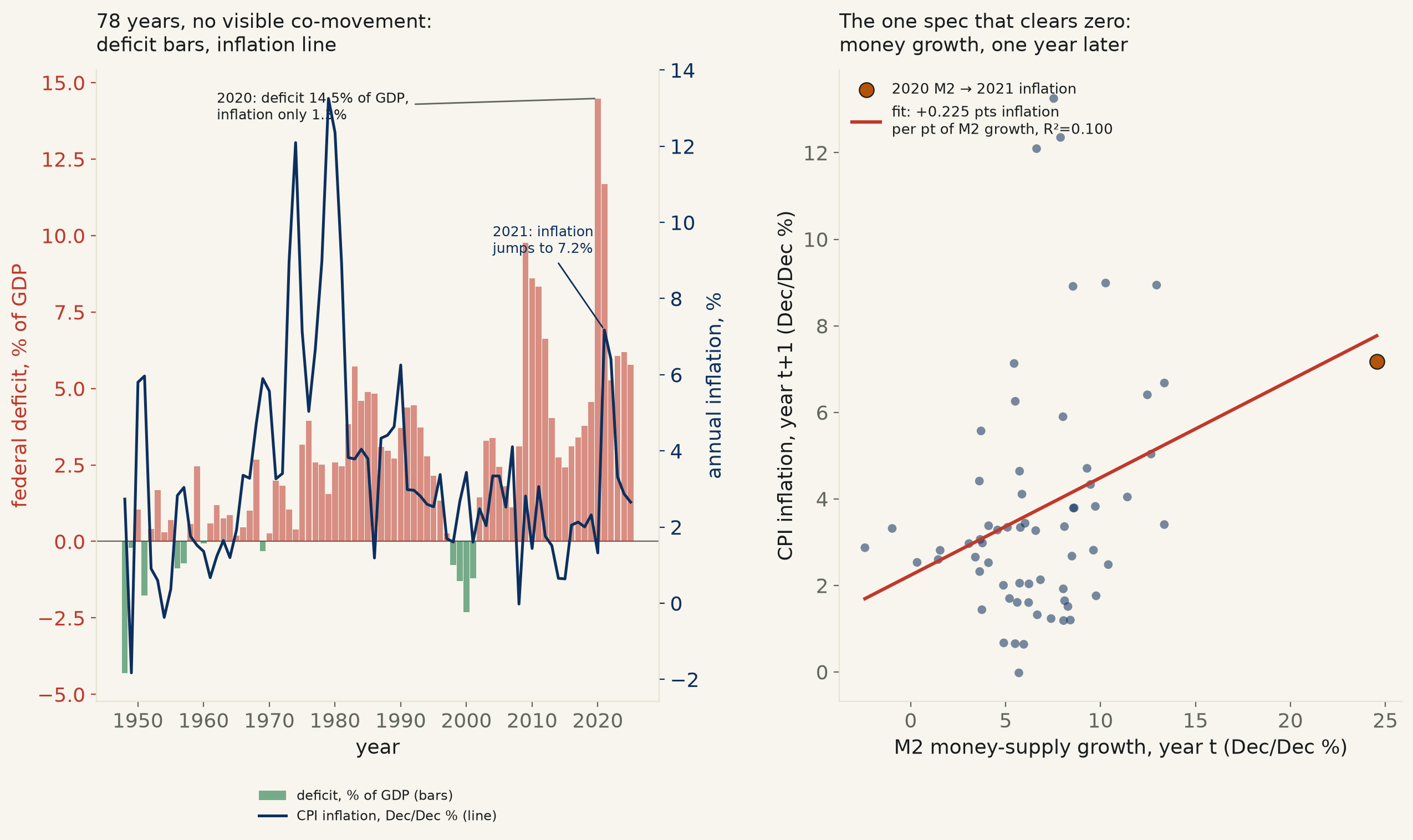
FRED’s own federal deficit, CPI, unemployment, and M2 money-stock series, 78 years, 1948–2025. The deficit itself vs. same-year inflation: +0.014, 95% CI [−0.150, +0.179] — contains zero, and stays there at ±1 and ±2-year lags, controlling for unemployment, and split at 1971’s end of the gold link. The actual “printing money” channel, M2 growth, does clear zero — but a year late: +0.225 points of next year’s inflation per point of M2 growth (CI [+0.135, +0.316], p<0.001), R²=0.10, surviving a bootstrap, a rank-correlation check, and dropping 2020. 2020’s record 14.5% deficit produced 1.3% inflation that year; 2020’s record 24.5% M2 growth showed up in 2021’s 7.2% instead.
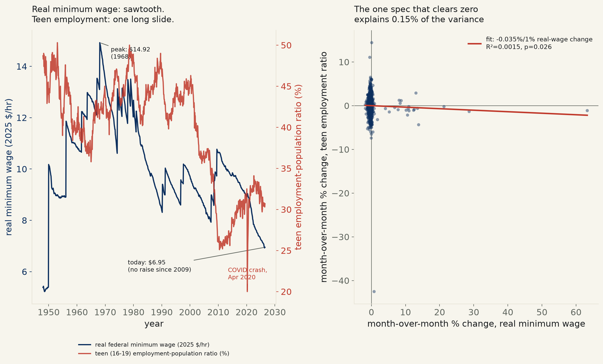
FRED’s own federal minimum wage, CPI, and CPS teen/prime-age employment ratios, 942 months, 1948–2026. The theoretically cleanest test — real minimum wage level vs. teen employment level, controlling for the decades-long trend both share — returns elasticity −0.058, 95% CI [−0.212, +0.096]: contains zero. Switch to month-to-month changes and a small negative effect clears zero under Newey-West, year-clustered, and bootstrap standard errors alike — but R²=0.0015, about one part in 700 of the variance. The real minimum wage peaked at $14.92/hr (2025 dollars) in 1968; after 17 years with no raise, it is worth $6.95 today.
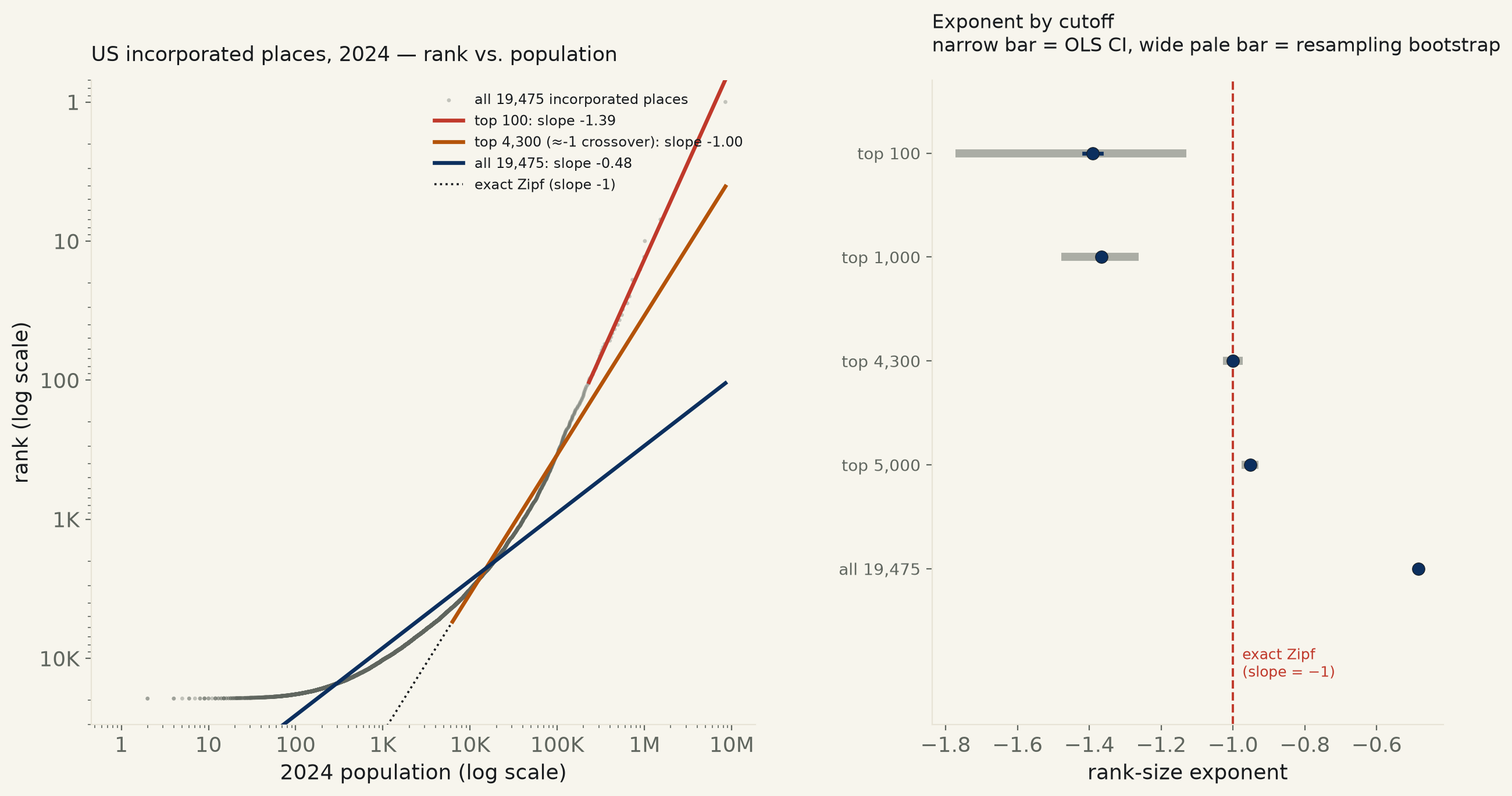
Every populated, legally incorporated US place, 2024 Census PEP estimates (19,475 places after excluding 4 with zero population). Rank-size exponent (log rank vs. log population): −1.39 for the top 100 (95% CI [−1.41, −1.37], bootstrap [−1.77, −1.13]) — steeper than Zipf’s textbook −1, both intervals excluding it. It flattens smoothly as the cutoff widens, crossing exactly −1.00 only in a narrow band near the 4,300th-largest place (95% CI [−1.005, −0.995]), then keeps flattening to −0.48 (CI [−0.487, −0.482]) across the full national list. R² stays above 0.87 at every cutoff — the fit looks clean throughout, even as the exponent it reports keeps moving.
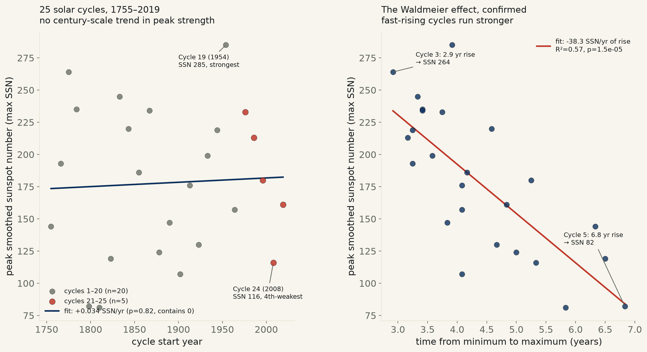
All 25 officially numbered solar cycles since 1755 (SIDC/SILSO & NOAA SWPC dating). Cycle length averages 11.03 years (95% CI [10.55, 11.52]) with no century-scale drift (95% CI on the trend [−0.008, +0.005] yr/yr, p=0.60). Peak sunspot number shows no long-run decline either (p=0.82) — nor do the 5 most recent cycles run weaker than the other 20 (p=0.90), despite Cycle 24’s real, named weakness (4th-weakest of 25). What is real: the Waldmeier effect — cycles that rise from minimum to maximum faster peak higher, −38.3 SSN points per extra year of rise, 95% CI [−52.8, −23.8], R²=0.57, p=1.5×10⁻⁵.
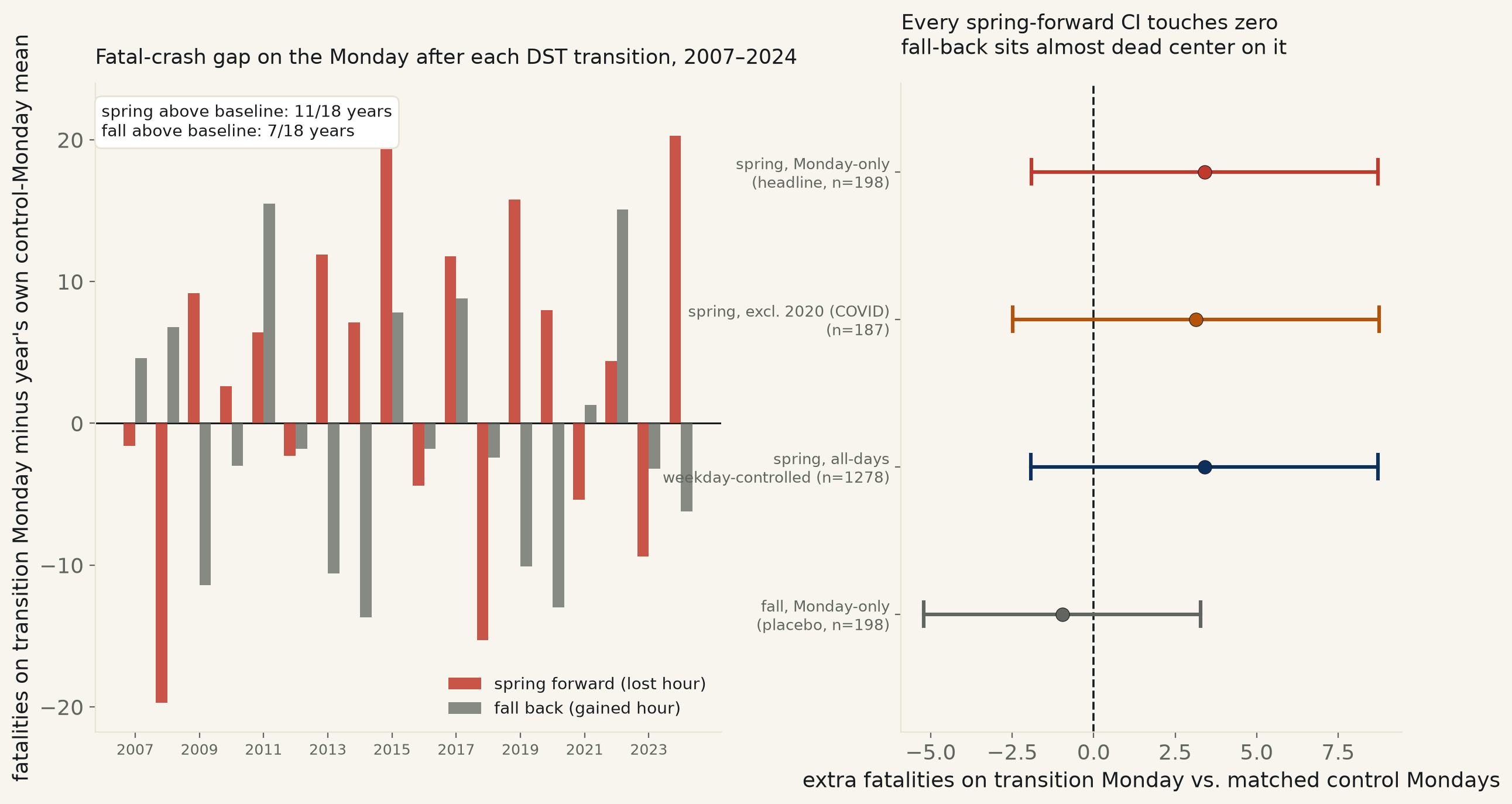
Every Monday within 5 weeks of all 18 US DST transitions since the modern rule began, NHTSA’s own fatal-crash microdata (FARS). The spring-forward Monday averages 84.2 fatalities vs. 80.8 on nearby control Mondays (+3.41, 95% CI [−1.92, +8.73], p=0.21, year-clustered) — the popular claim’s own direction, not far from significant, and still crossing zero. A 4,000-draw bootstrap lands closer: 90.8% of resamples are positive, short of the 95% the desk requires. The fall-back Monday, gaining an hour instead of losing one, comes back almost dead center on zero (−0.96, CI [−5.21, +3.29], p=0.66) — the internal placebo the spring result needs and doesn’t get to lean on.
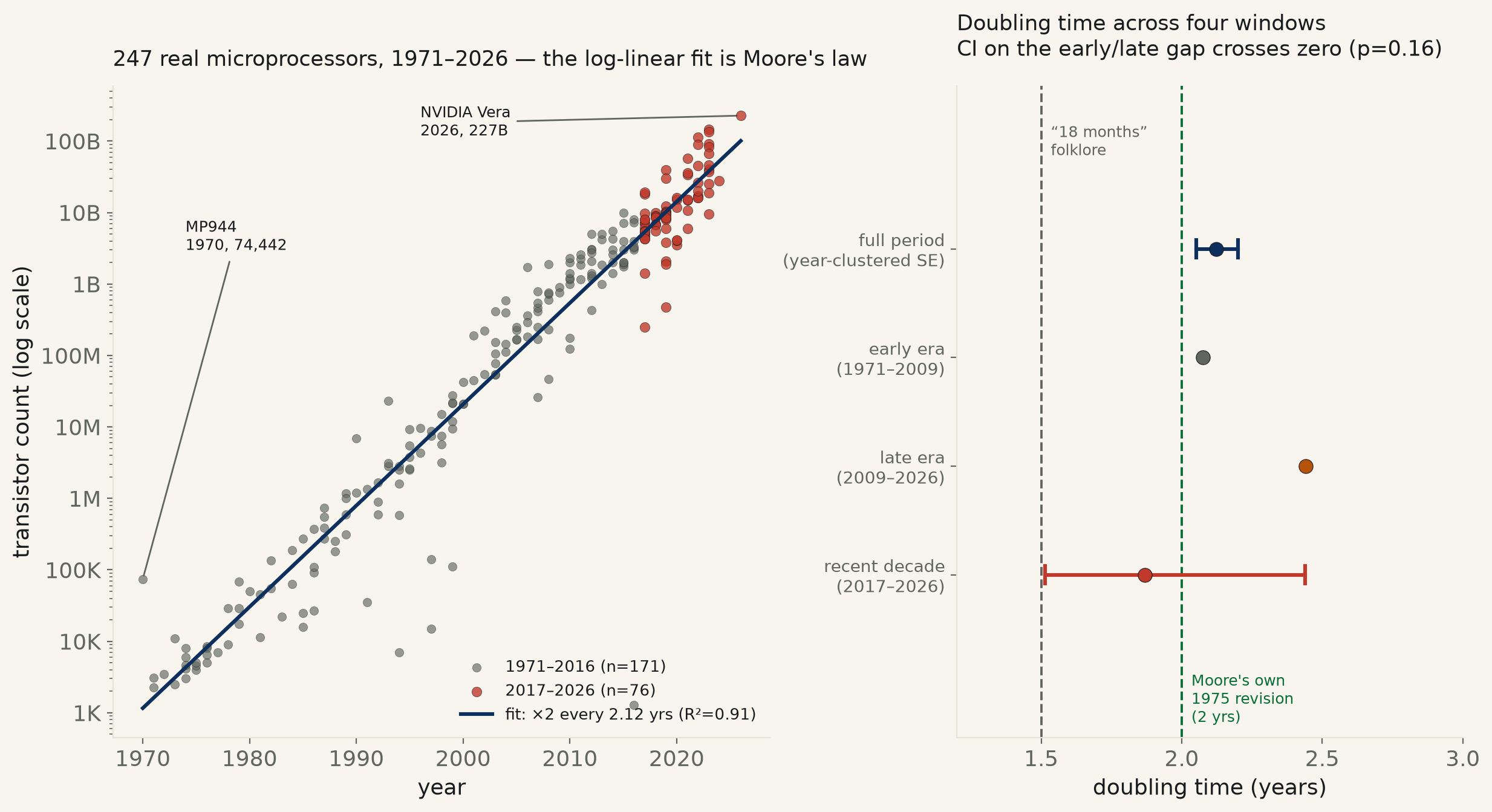
Every microprocessor Wikipedia’s own transistor-count table lists with a year and a count, 247 chips, 1970–2026. Doubling time: 2.12 years (95% CI [2.05, 2.20], R²=0.915) — excluding both the popular “18 months” folklore and Moore’s own revised “two years” prediction. Split at the data’s own median year (2009): the point estimate for a slowdown exists (2.08→2.44 yrs) but the interaction test’s CI crosses zero (p=0.16) — the desk can’t confirm the law itself bent. What does change: R² collapses 0.88→0.35, likely because “a microprocessor” stopped meaning one thing.
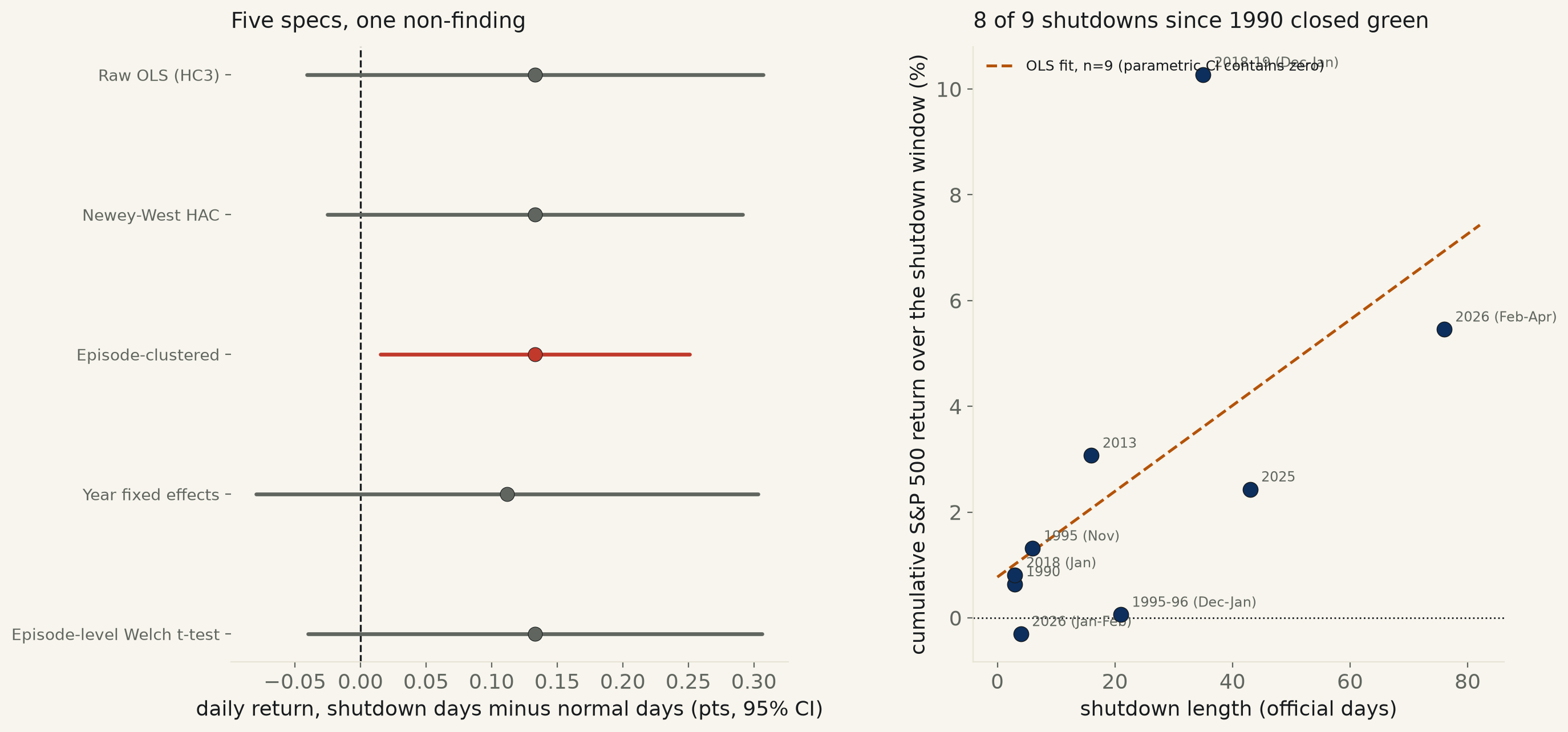
Nine federal shutdowns since 1990, S&P 500 daily closes. Three of four day-level specifications find no detectable difference between shutdown-day and normal-day returns (raw OLS, 95% CI [−0.04, +0.31] pts/day, p=0.13); the one exception (episode-clustered SEs) narrowly excludes zero but rests on just 9 shutdown episodes. Concretely, 8 of 9 shutdowns since 1990 closed with the index higher than when they started — only the 4-day Jan–Feb 2026 lapse closed lower. A duration-vs-return regression (n=9) disagrees with itself: parametric CI contains zero, a 4,000-draw bootstrap narrowly excludes it — reported as an unresolved near-miss, not a finding.
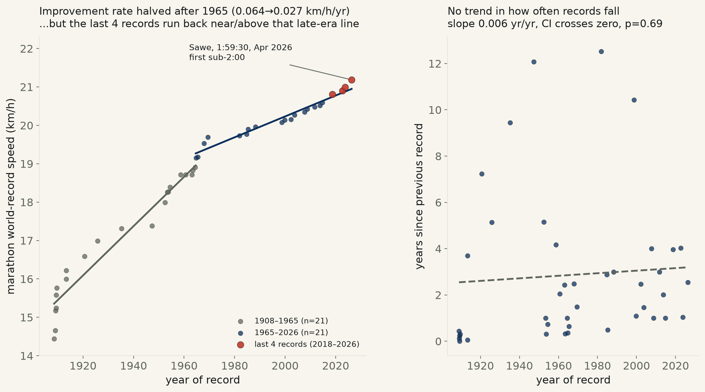
Cleaned to the true best-ever-to-date progression (42 men’s records, 1908–2026), the marathon world record’s improvement rate really did halve: +0.064 km/h per year before 1965 vs. +0.027 after (95% CI on the gap [−0.046, −0.028], p<10−9) — the “humans are near their limit” story, confirmed, for the 20th century. But the last 9 records (2006–2026) improved at +0.042 km/h/yr, almost back to the century average, and Sabastian Sawe’s 1:59:30 (Apr 2026, the first sub-2:00) lands 1.1% above where the post-1965 line predicted, not below it. The women’s record shows the identical halve-then-catch-up shape. No trend in how often records fall either (p=0.69).
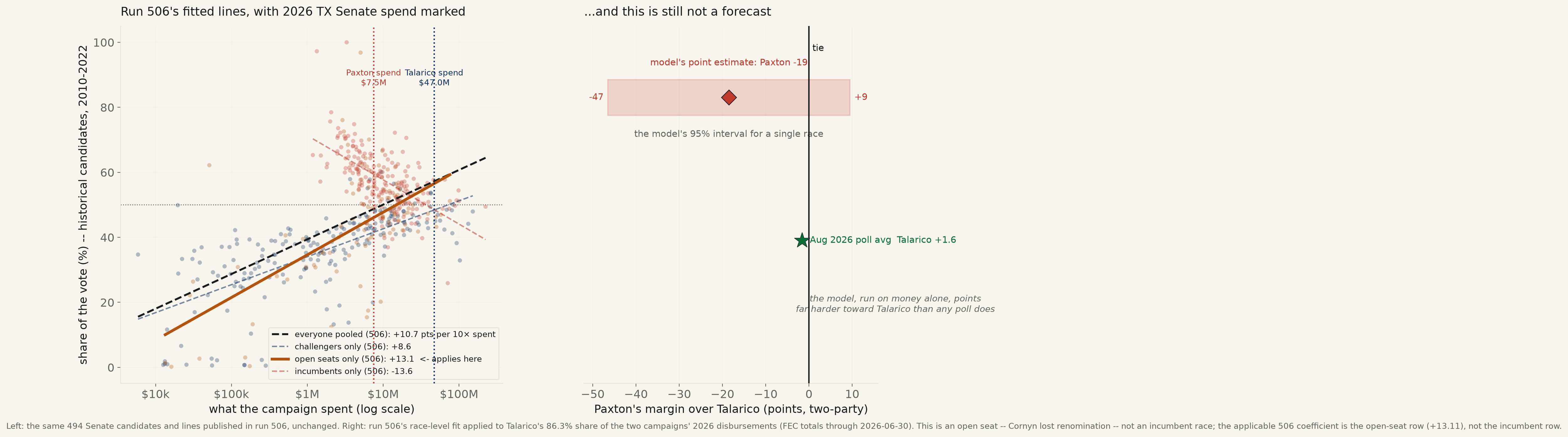
Run 506 fitted a Senate open-seat coefficient of +13.11 points per tenfold spent and published it. This run applies it, unrefit, to a live race: Cornyn lost renomination to Paxton in the May 2026 GOP runoff, so by the FEC’s own coding this is an open seat, not an incumbent race. Talarico’s 86.3% share of the two campaigns’ money returns a point estimate of Paxton −18.5 and a 95% interval 56.0 points wide [Paxton −46.5 to +9.5] — far outside the August 2026 polling average (Talarico +1.6). Reported Musk/America PAC spending ($100–200M, national, no Texas-specific figure reported) sits entirely outside what any of run 505/506’s coefficients were fitted on — candidate committee money only.
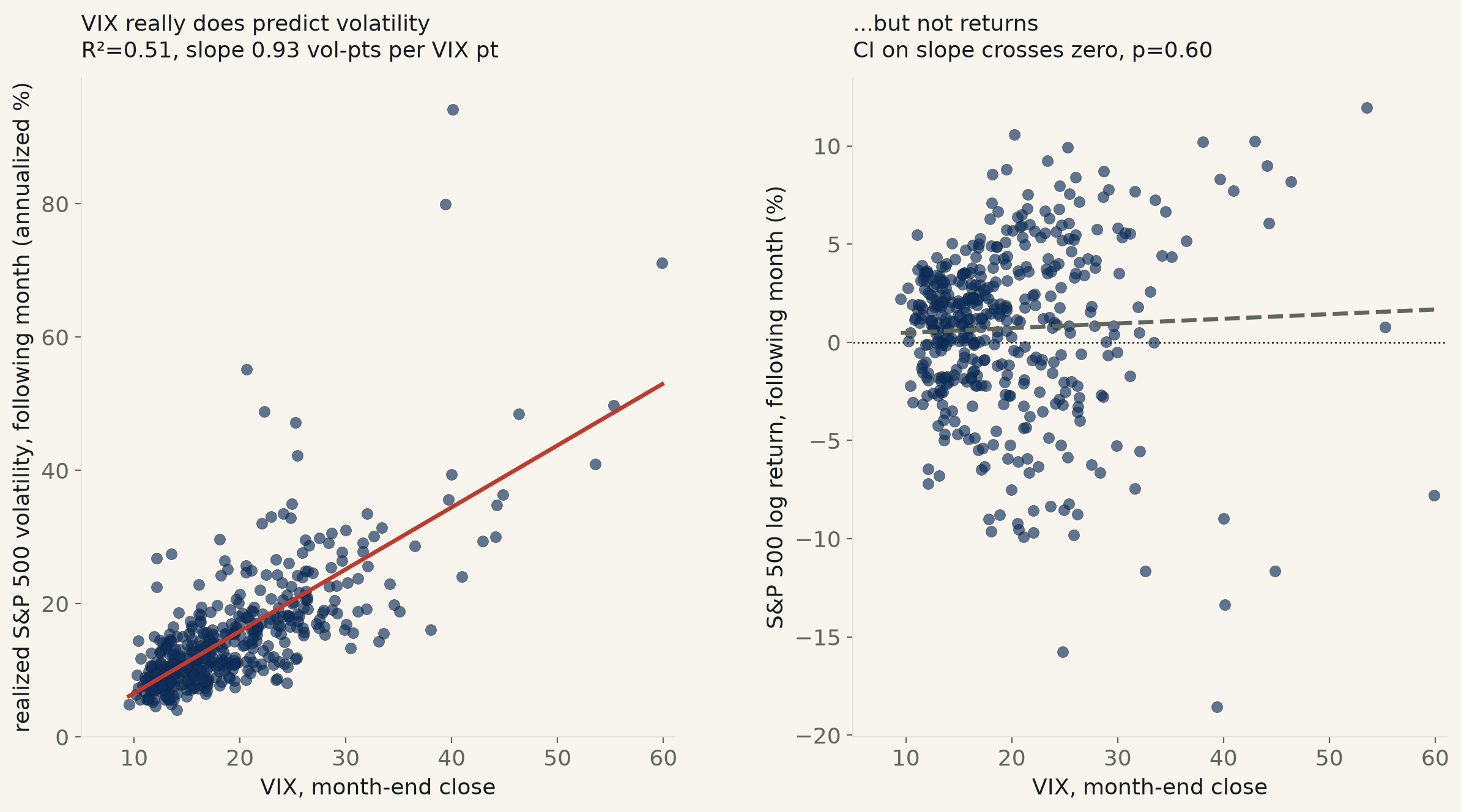
438 non-overlapping months since 1990, the VIX’s own month-end close (Yahoo Finance) paired with the S&P 500’s realized volatility and log return the following month. The VIX prices next month’s volatility well: +0.93 vol-points per VIX point (95% CI [+0.77, +1.09], R²=0.51, p<10−27). It has nothing to say about next month’s return: +0.02% per VIX point (CI [−0.07, +0.11], R²=0.0017, p=0.60). And it is a biased predictor even of the thing it is good at — the VIX overshoots the realized volatility that follows it by +4.10 points a year on average (CI [+3.47, +4.73], true in 83% of months), the volatility risk premium option sellers are paid to bear.
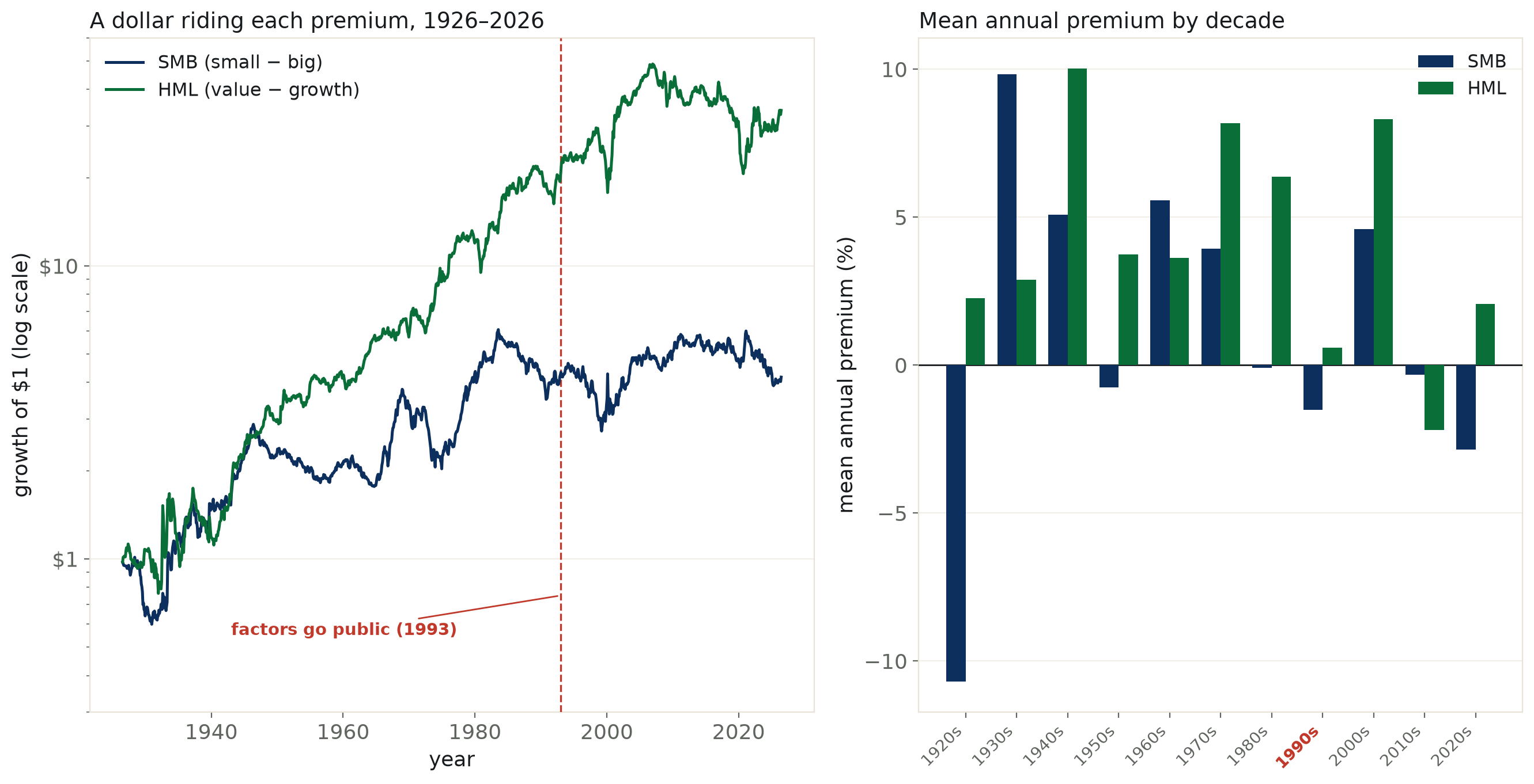
SMB and HML are the literal, tradeable size and value premiums Fama and French published in 1993, tracked monthly ever since. Regressing each factor’s annual return on the calendar year across 99 complete years: SMB −0.056 pts/yr (95% CI [−0.140, +0.028]), HML −0.050 pts/yr (CI [−0.145, +0.045]) — both contain zero, though a 4,000-draw bootstrap puts 90% and 82% of resampled slopes below it. Split flatly at 1993 (the year the factors went public): SMB’s mean annual premium falls from +3.16% to +0.17%, HML’s from +5.37% to +2.41% — real-looking drops whose own bootstrap intervals still contain zero. What needs no interval: a dollar in SMB is worth less today than it was the day before the 1993 cutoff ($4.26 → $4.17), and the last full decade averaged −2.32%/yr for size, +0.37%/yr for value.
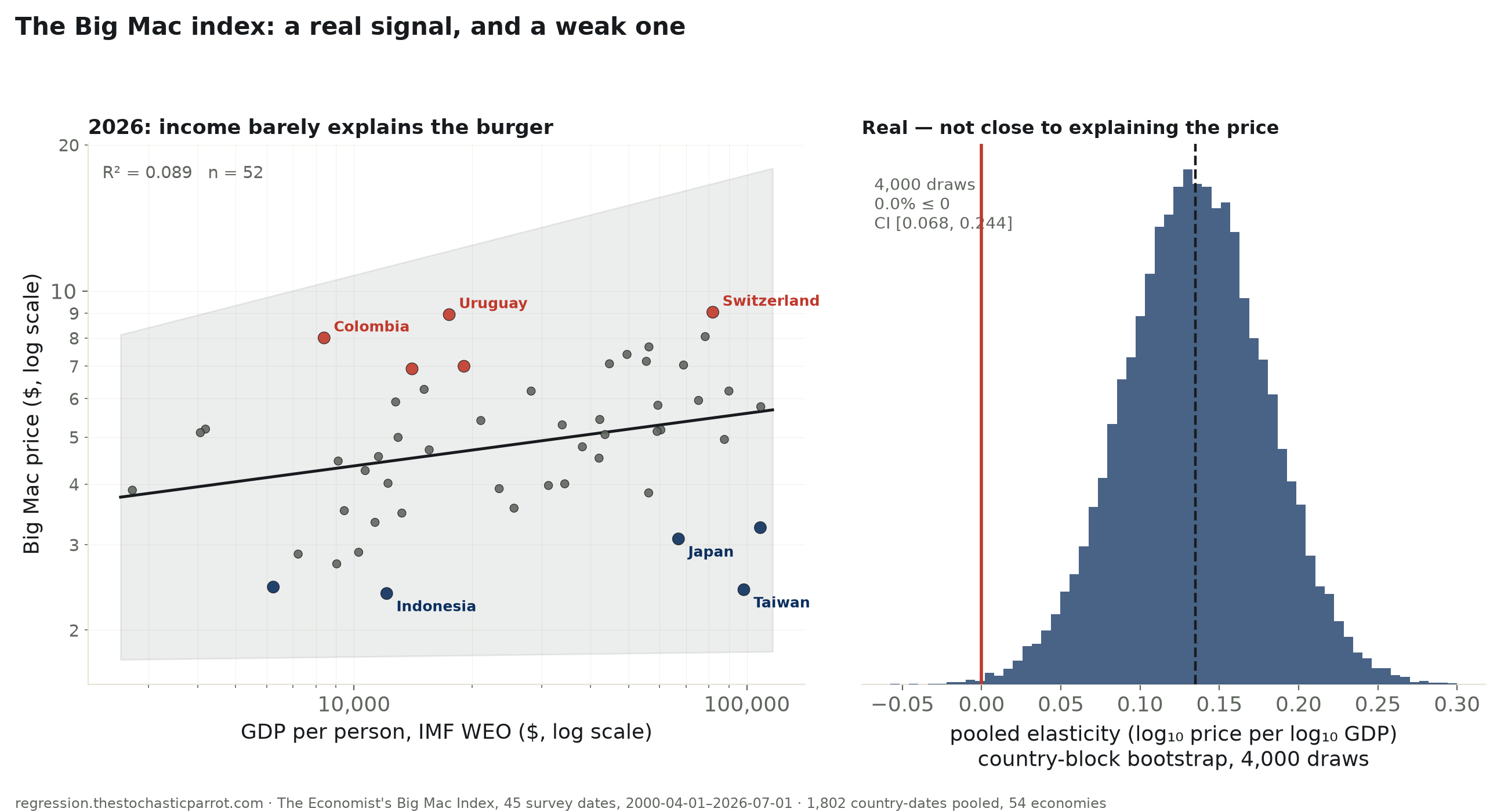
The Economist’s own “GDP-adjusted” Big Mac index is a fitted line — local dollar price regressed on GDP per person. Refit it independently, pooled across 45 survey dates and 54 economies since 2000 (1,802 country-dates, country-clustered SEs): the slope is real, +0.135 log₁₀ price per log₁₀ GDP (95% CI [+0.046, +0.223], 4,000-draw bootstrap 0% at or below zero) — but R² = 0.164. On the newest snapshot alone, R² = 0.089. Three rich Asian economies — Taiwan, Japan, Hong Kong — price a burger 42–58% below what their income implies; China sits 18% under its own line, a mild version of the “undervalued yuan” story, not the dramatic one. The elasticity itself has not moved since 2000 (CI on the 26-year trend contains zero).
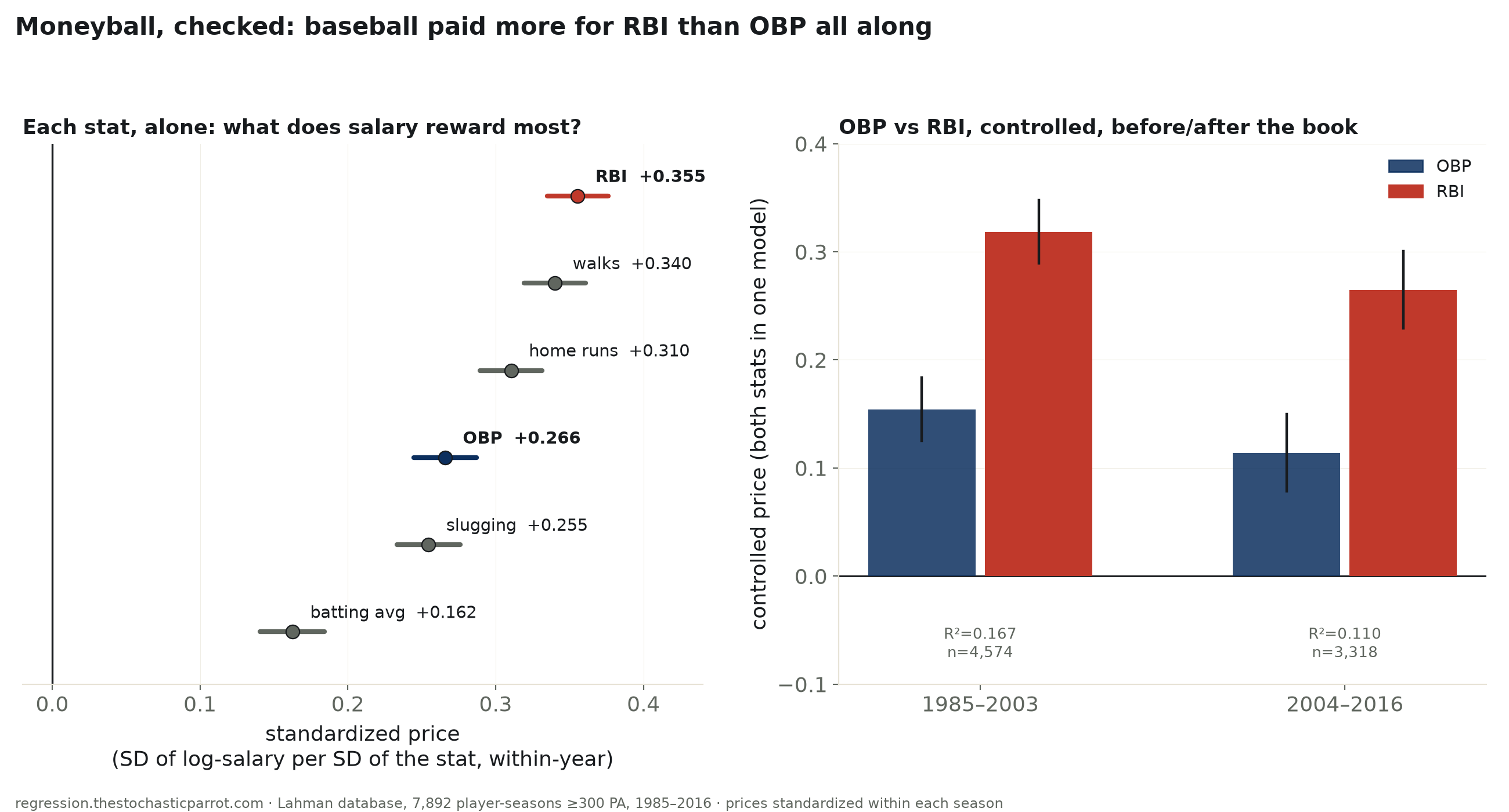
7,892 qualified hitter-seasons (≥300 plate appearances), 1985–2016 — the full span the sport’s own salary database covers. Standardized within each season (so 32 years of salary inflation cannot fake a trend), on-base percentage alone prices at +0.266 SD of log-salary per SD of OBP — fifth of six batting stats tested. RBI prices highest, at +0.355. Put both in one model and RBI keeps more than double OBP’s controlled price (+0.296 vs +0.137), and home runs add nothing once RBI is already in. After Michael Lewis’s 2003 book, RBI’s controlled premium measurably shrank (−0.054, CI excludes zero) — but OBP’s own price did not measurably rise, and the whole model got worse at explaining salary (R² 0.167→0.110). The book’s own hero makes the point concretely: Scott Hatteberg’s 2002 OBP ranked in the 84th percentile of that year’s qualifiers; his salary ranked in the 31st.
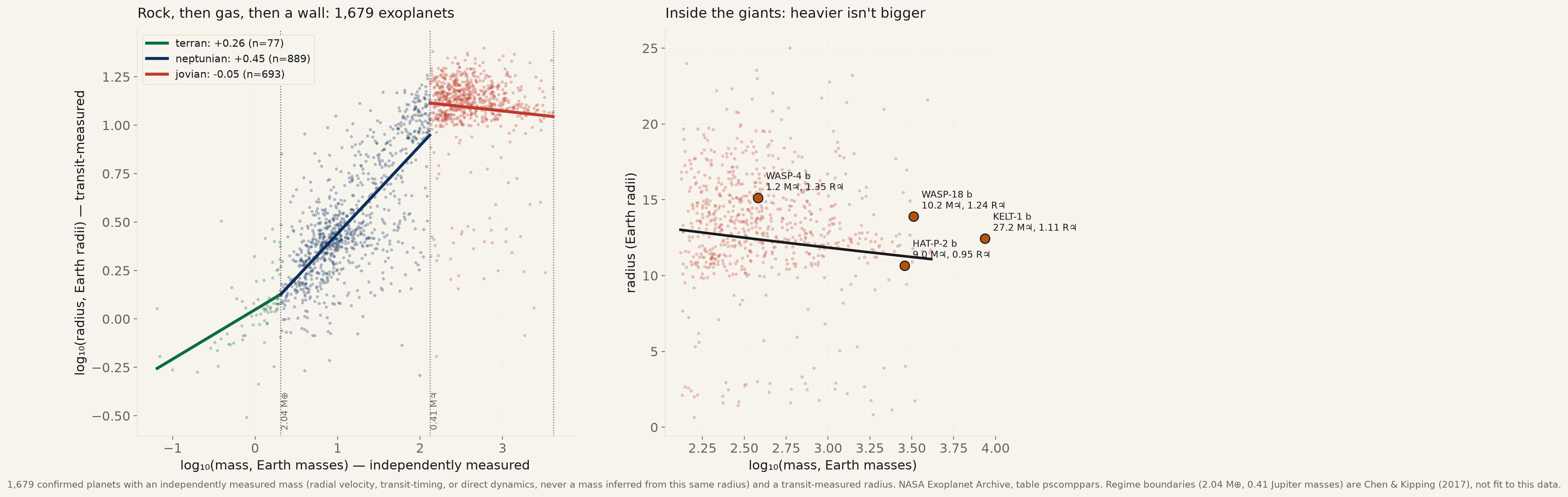
1,679 confirmed exoplanets with an independently measured mass and a transit-measured radius (NASA Exoplanet Archive) — after throwing out the 47.5% of the archive’s mass-radius rows where the mass was computed FROM the same radius, a circularity that alone produces R²=0.97. Rocky worlds under 2.04 Earth masses: slope +0.26 (CI excludes zero). Add a gas/ice envelope (up to 0.41 Jupiter masses): +0.45, steeper — CI excludes zero cleanly, 0% of bootstrap resamples on the wrong side. Past that, among 693 gas giants up to the brown-dwarf line: −0.047 — the parametric interval barely excludes zero, but a 4,000-draw bootstrap puts 95.8% below zero and its own interval touches zero. WASP-4 b (1.2 Jupiter masses) to KELT-1 b (27.2 Jupiter masses, 23× the mass): a smaller radius.
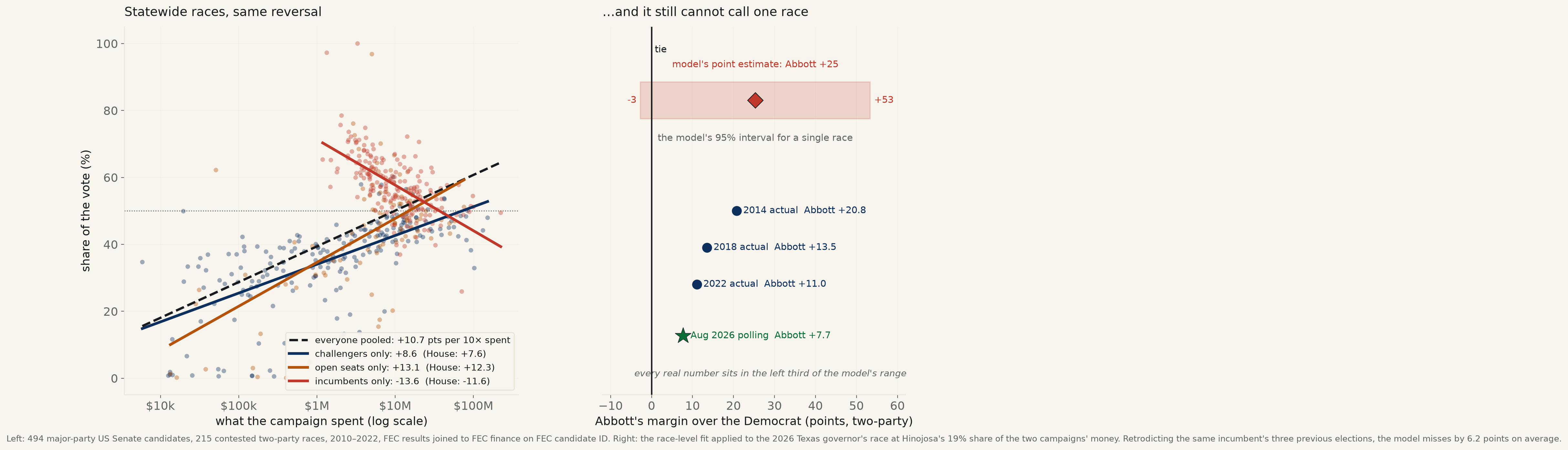
Run 505 found that campaign spending tracks vote share hard across candidates and runs backwards inside the incumbents — on 2,263 US House races. The obvious objection was scale, so the desk refit the whole thing on the closest federal analogue to a statewide office: 494 major-party US Senate candidates, 215 contested races, 2010–2022, joined the same way on the FEC’s own candidate ID. It replicates line for line — pooled +10.67, challengers +8.60, open seats +13.11, incumbents −13.62 (CI [−16.19, −11.04]) against −11.56 in the House, with 4,000 bootstraps below zero every time. Money is also less decisive as the electorate grows: the bigger spender wins 77.2% of Senate races vs 89.0% of House races, and just 65.1% of Senate open seats. Then the model was aimed at a live election — the 2026 Texas governor’s race — and made to retrodict the same incumbent’s three previous elections first: it misses by 6.2 points on average, in both directions, and returns a 2026 interval 56 points wide containing a landslide and a defeat. A relationship solid across two thousand races and useless for the next one.
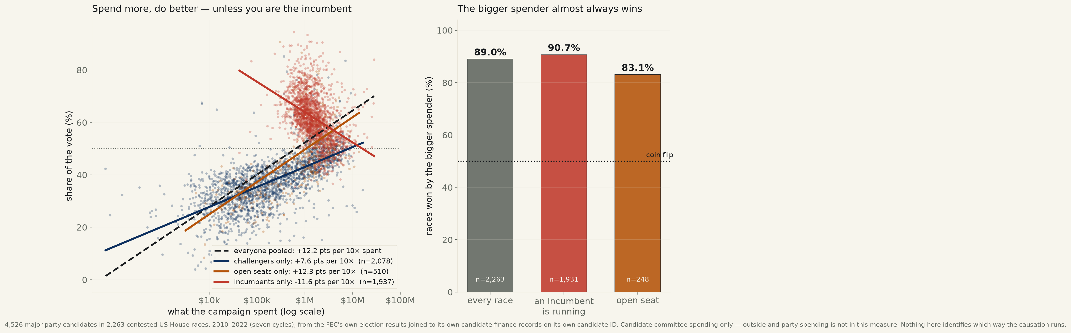
5,405 major-party US House candidates across seven post-Citizens United cycles, 2010–2022, built by joining the FEC’s own election results to the FEC’s own campaign finance records on the FEC’s own candidate ID — an exact join, no name matching. Pooled, the slogan holds: +12.21 points of vote share per tenfold spent (95% CI [+11.77, +12.65], R²=0.395), and the bigger spender takes 89.0% of contested races. Run the identical fit inside each group and one line reverses: challengers +7.62, open seats +12.35, incumbents −11.56 (CI [−12.71, −10.41]) — an incumbent who spends ten times as much does about twelve points worse, and 4,000 bootstrap refits put that below zero every time. Both campaigns’ spending in one model points down together. The money is a smoke alarm, not a fire engine — and in open seats, where incumbency is out of the way, the bigger spender wins least often of all (83.1%).
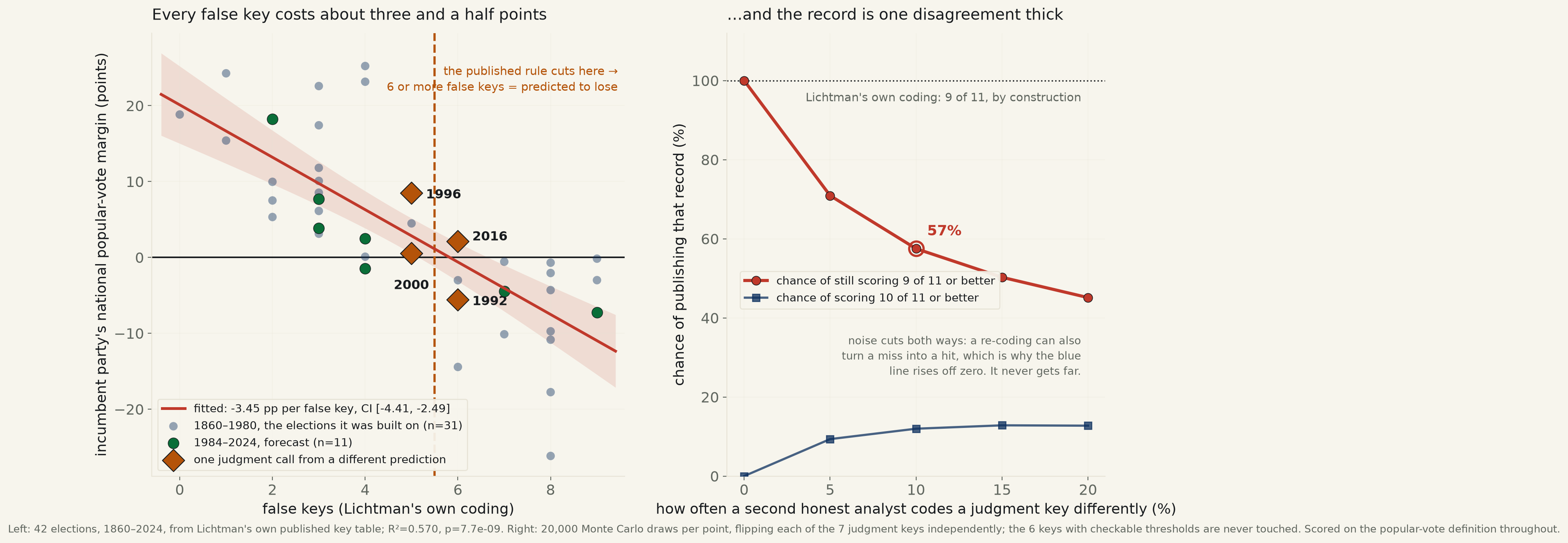
42 US presidential elections, 1860–2024, scored under Allan Lichtman’s 13 Keys (6 objective counts, 7 judgment calls) against the incumbent party’s popular-vote margin. The model works: R²=0.57, p=8×10⁻⁹, and the published cutoff of 6 false keys sits close to what the data itself crosses zero at — 5.5 to 6.5 keys depending on the specification. But 7 of the 13 keys require a judgment call, and a coder-disagreement simulation shows the model’s celebrated “9 or more correct every time since 1984” record is fragile: at just a 10% chance any one judgment key flips coder-to-coder, the odds of still landing 9+ correct fall from 100% to 57%.
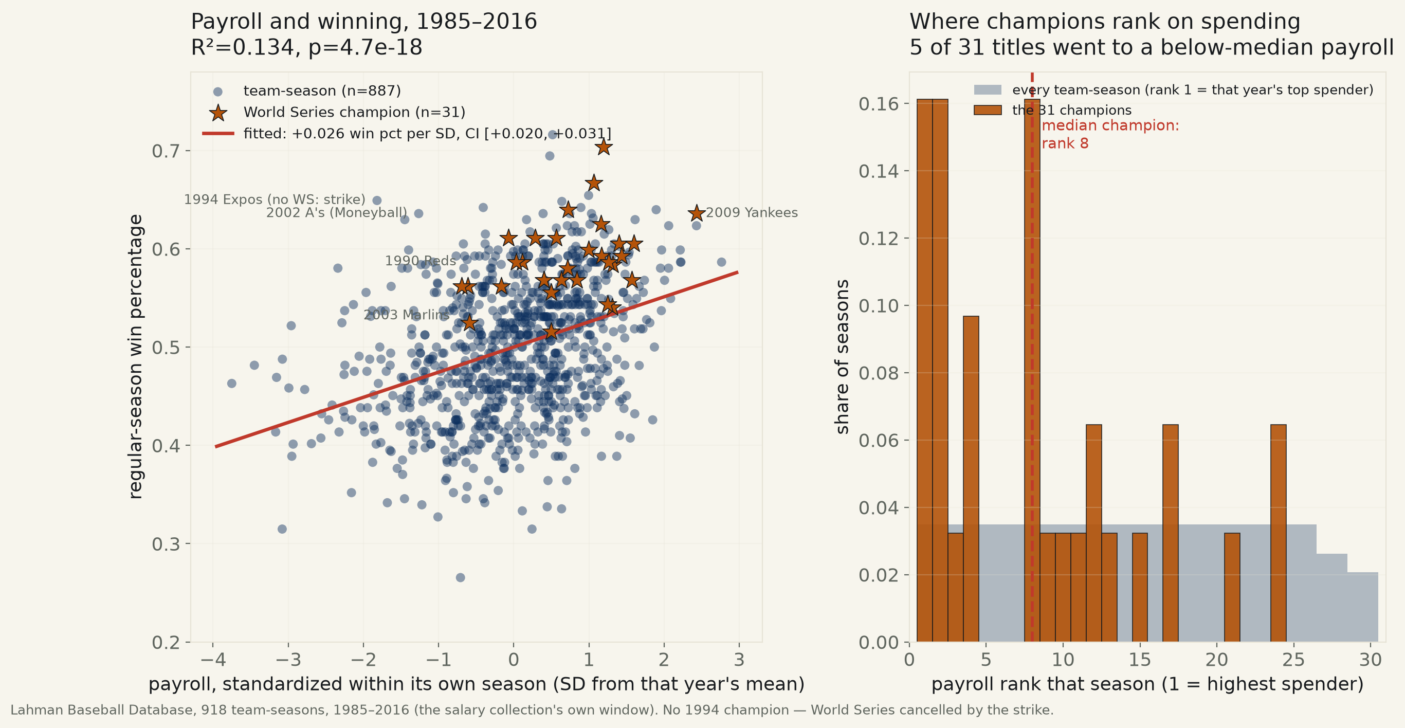
918 MLB team-seasons, 1985–2016 (Lahman Baseball Database). Payroll, standardized within its own season, predicts win percentage: +0.026 per SD (95% CI [+0.020, +0.031], R²=0.134) — real, and explains about an eighth of the variance. Championship odds rise 2.67× per SD of payroll (CI [1.87, 3.80], excludes 1). The median champion ranked 8th in payroll that season, against a league median of 15th — but 5 of 31 titles went to a below-median payroll anyway, and the relationship did not weaken after MLB's 2003 luxury tax.
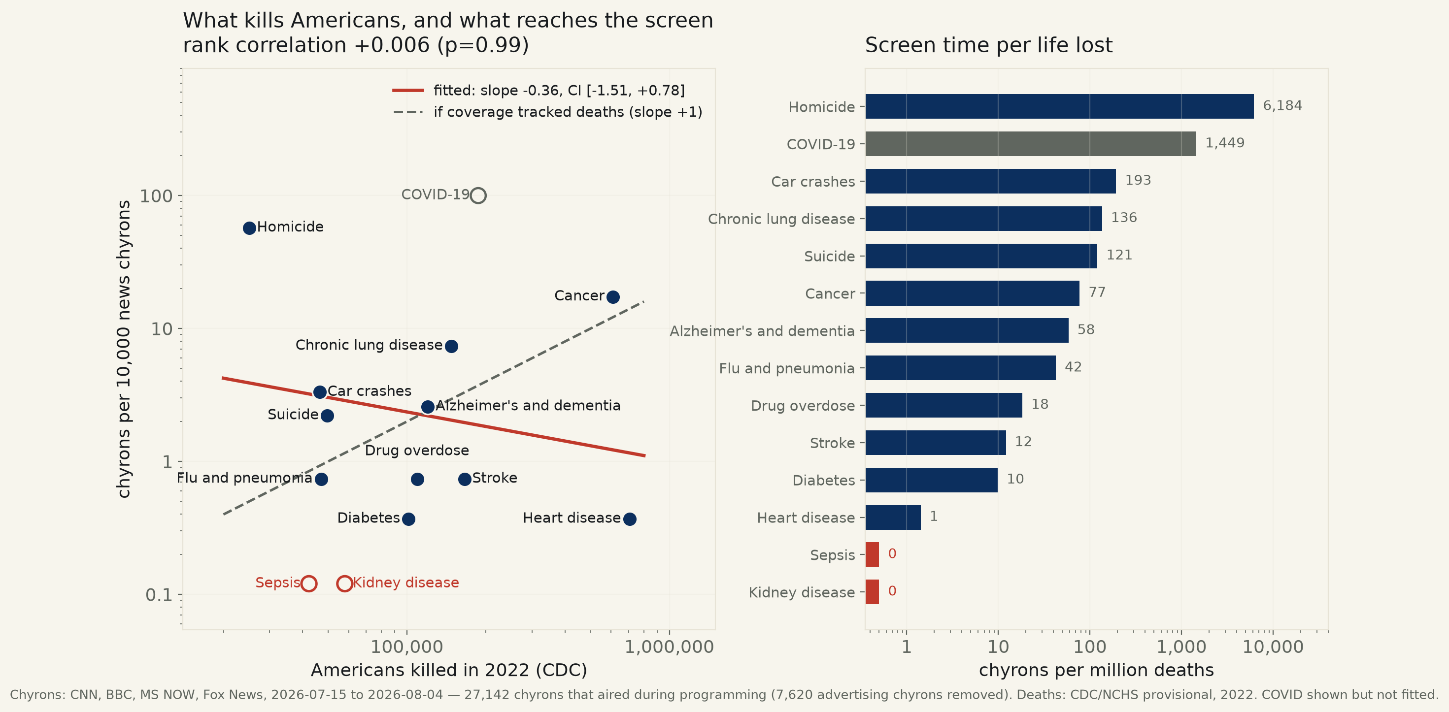
27,142 chyrons that aired during programming on CNN, BBC, MS NOW and Fox News, 2026-07-15 to 2026-08-04, matched against CDC’s own count of what killed Americans. Heart disease killed 704,786 people and reached the screen once. Homicide killed 28× fewer and reached it 155 times. Across fourteen causes the rank correlation between deaths and coverage is +0.006 (p=0.99); the fitted slope’s 95% CI contains zero and excludes +1 — the desk can rule out coverage tracking mortality, and cannot distinguish it from unrelated. Sepsis and kidney disease, 100,366 deaths between them, were named zero times.
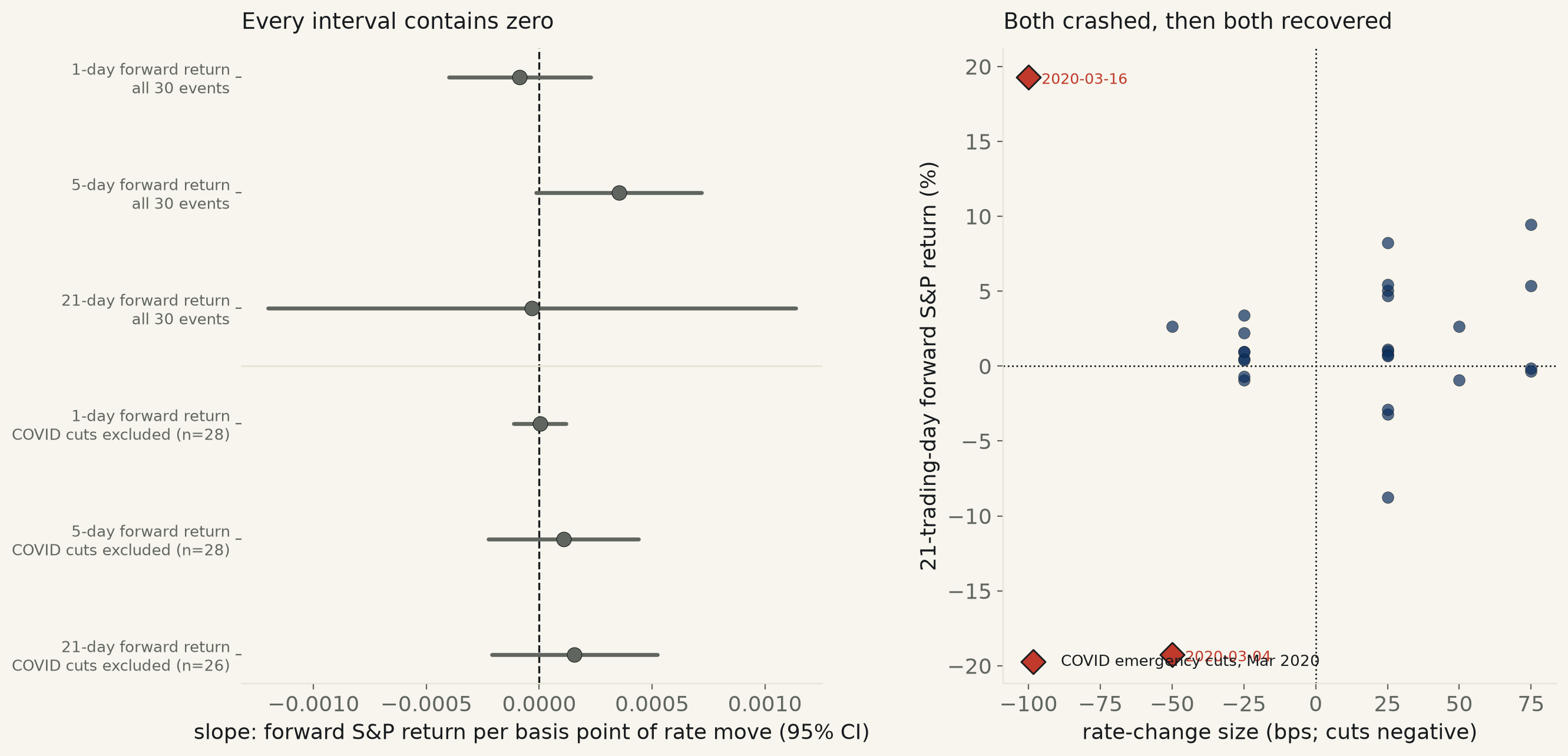
30 Fed rate-change decisions since 2016 (19 hikes, 11 cuts), read directly off FRED’s own daily federal-funds target-range series, paired with S&P 500 forward returns at 1, 5, and 21 trading days. No horizon shows a cut predicting a bigger rally — every 95% CI contains zero. The closest thing to a signal (5-day, p=0.06) runs the wrong direction and turns out to be two data points from a single week in March 2020: exclude just the two COVID emergency cuts and every slope moves further from significance, not closer.
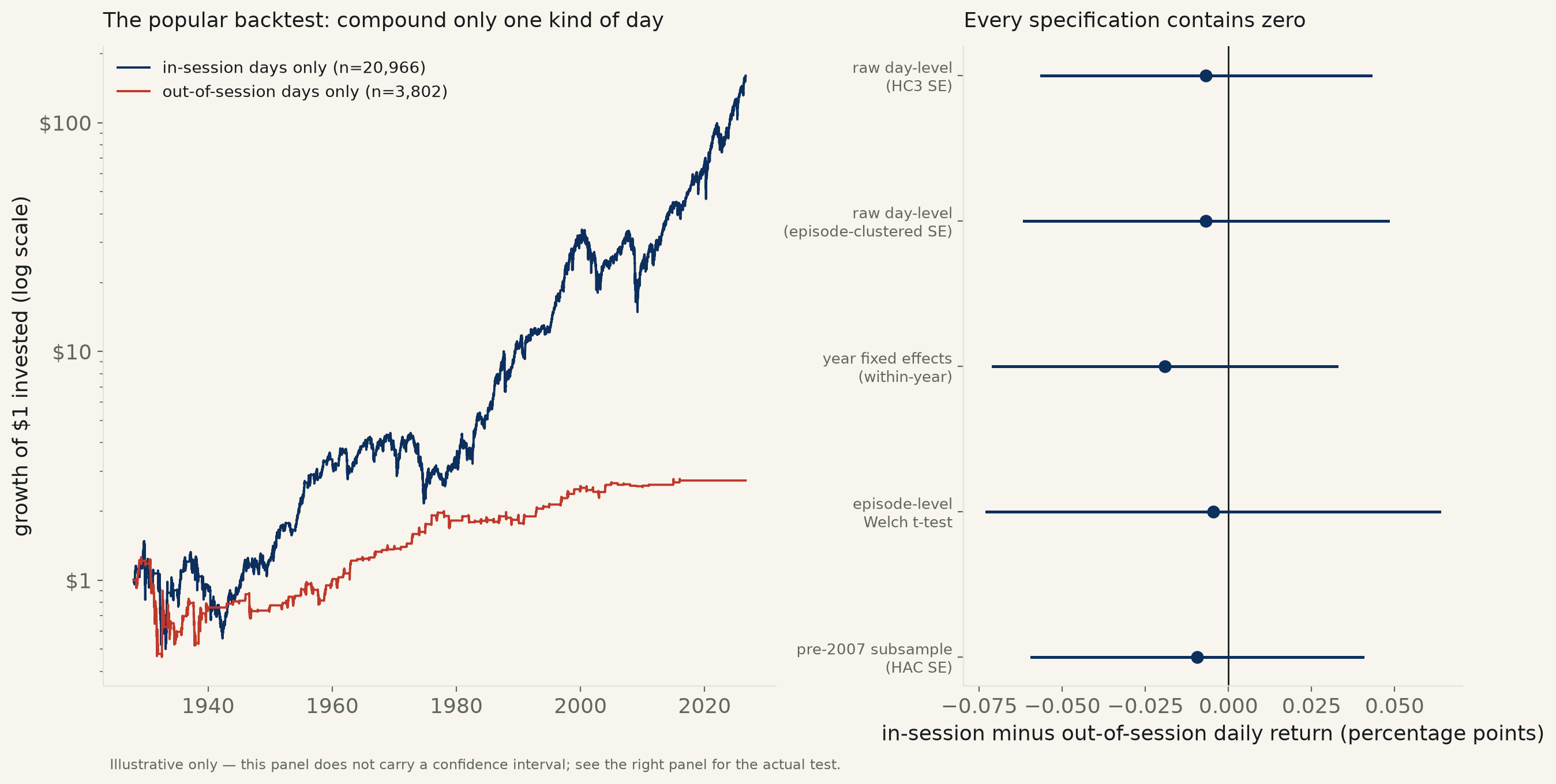
24,768 S&P 500 trading days, 1928–2026, classified by senate.gov’s own record of every session’s convening and adjournment date. Raw daily return: +0.031% in session vs +0.037% out — five separate tests of that gap (raw, HAC, episode-clustered, year fixed effects, episode-level t-test) all return a 95% CI that contains zero. Compound only the in-session days and only the out-of-session days separately, though, and $1 grows to $161 vs $2.73 — a trap: in-session days outnumber out-of-session days 5.5 to 1, mostly because Congress stopped formally adjourning after ~2007.
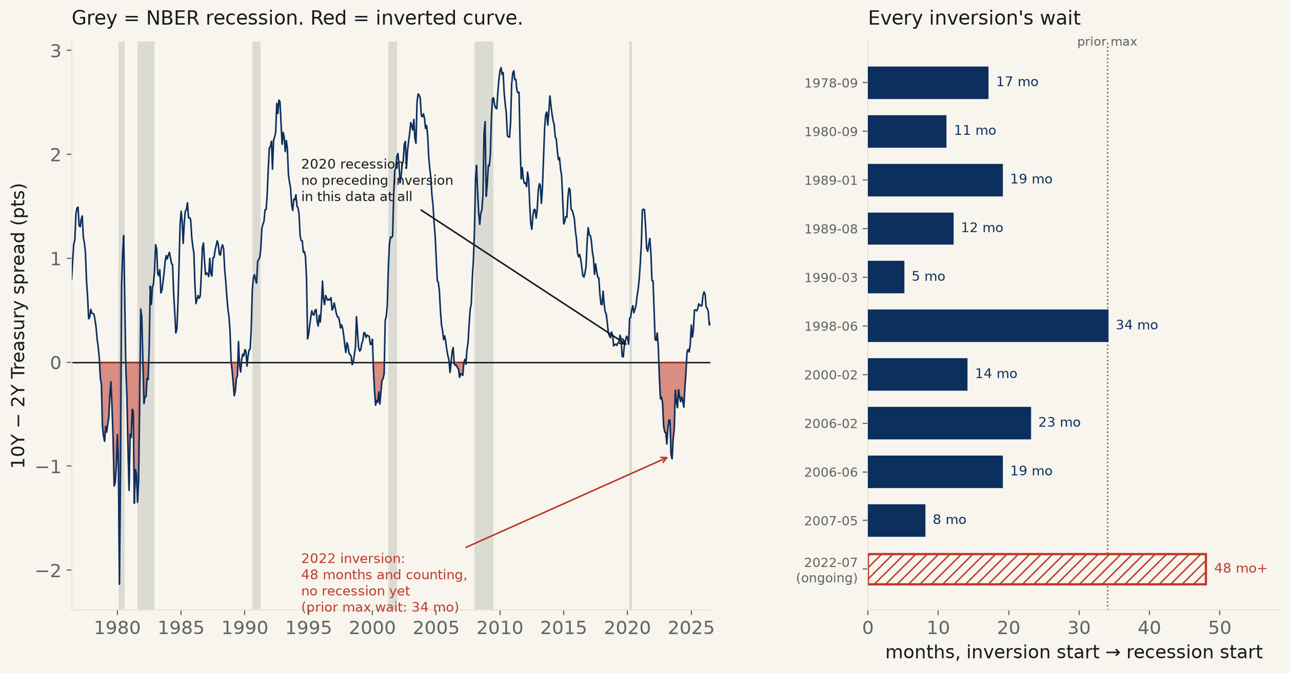
FRED, 1976–2026, 602 months. Every month the curve was inverted, a recession followed within a year 50.5% of the time, vs 15.1% when it wasn’t (95% CI on the gap [+27.1, +43.8] pts, excludes zero) — a real, if noisy, signal (R²=0.11; overlapping 12-month windows mean the interval is optimistic). The clean pattern breaks twice: the 2020 recession arrived with no preceding inversion at all in this data, and the curve that inverted in July 2022 has now gone 48 months without a recession — longer than any of the ten resolved inversions on record (previous max: 34).
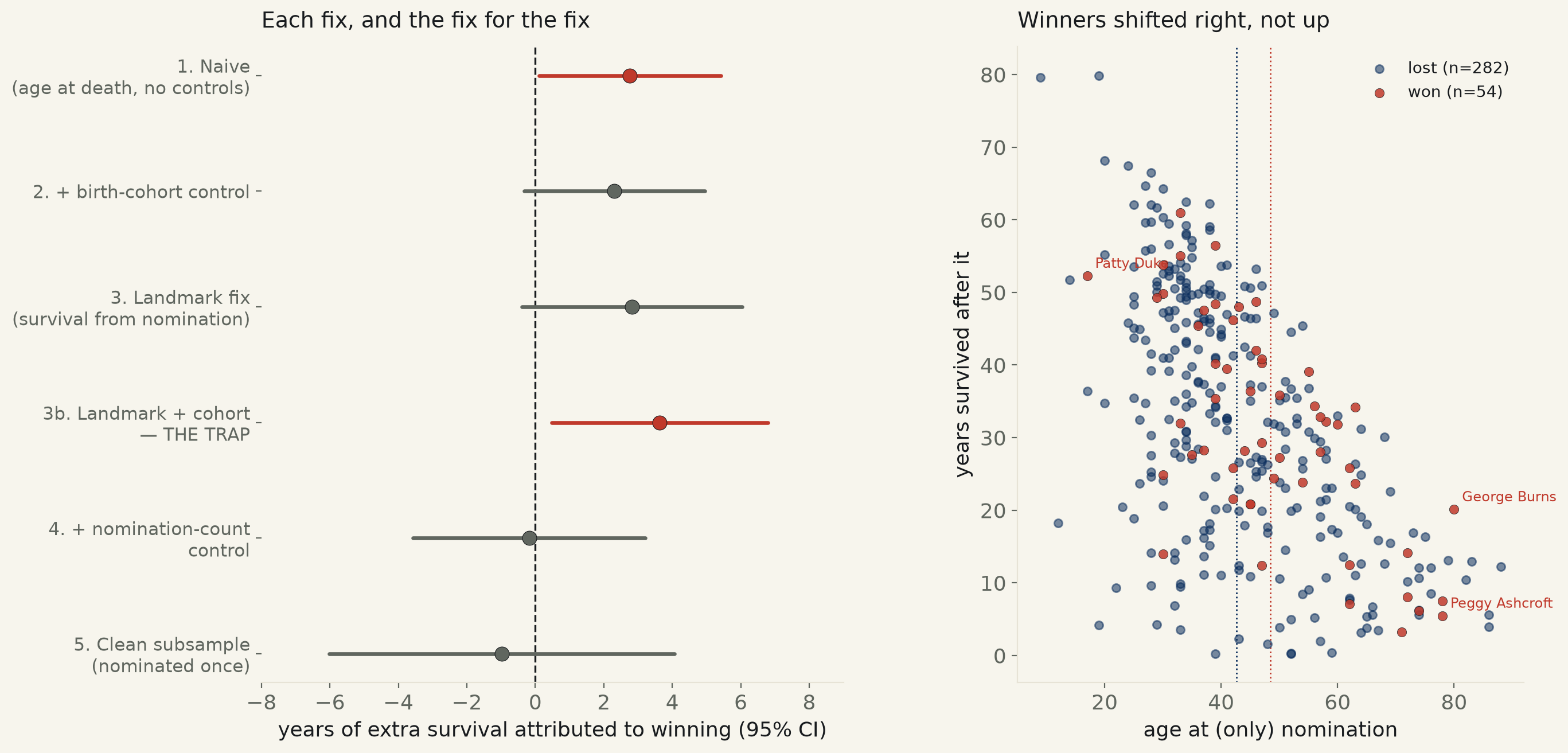
522 deceased Academy Award acting nominees (Wikidata, four categories, 1928–2026). Naive claim replicates: winners’ age at death runs +2.76 years higher (95% CI [+0.11, +5.41], barely excludes zero) — matching a famous 2001 paper. The textbook fix for immortal-time bias (measure survival from nomination, not birth) makes the estimate look stronger, not weaker: +3.64 years, CI [+0.48, +6.79]. The trap: winning is entangled with nomination count, itself just a symptom of a long career. Control for it and winning explains nothing — −0.18 years, CI [−3.58, +3.21], dead center on zero — confirmed in the clean one-shot-nominee subsample.
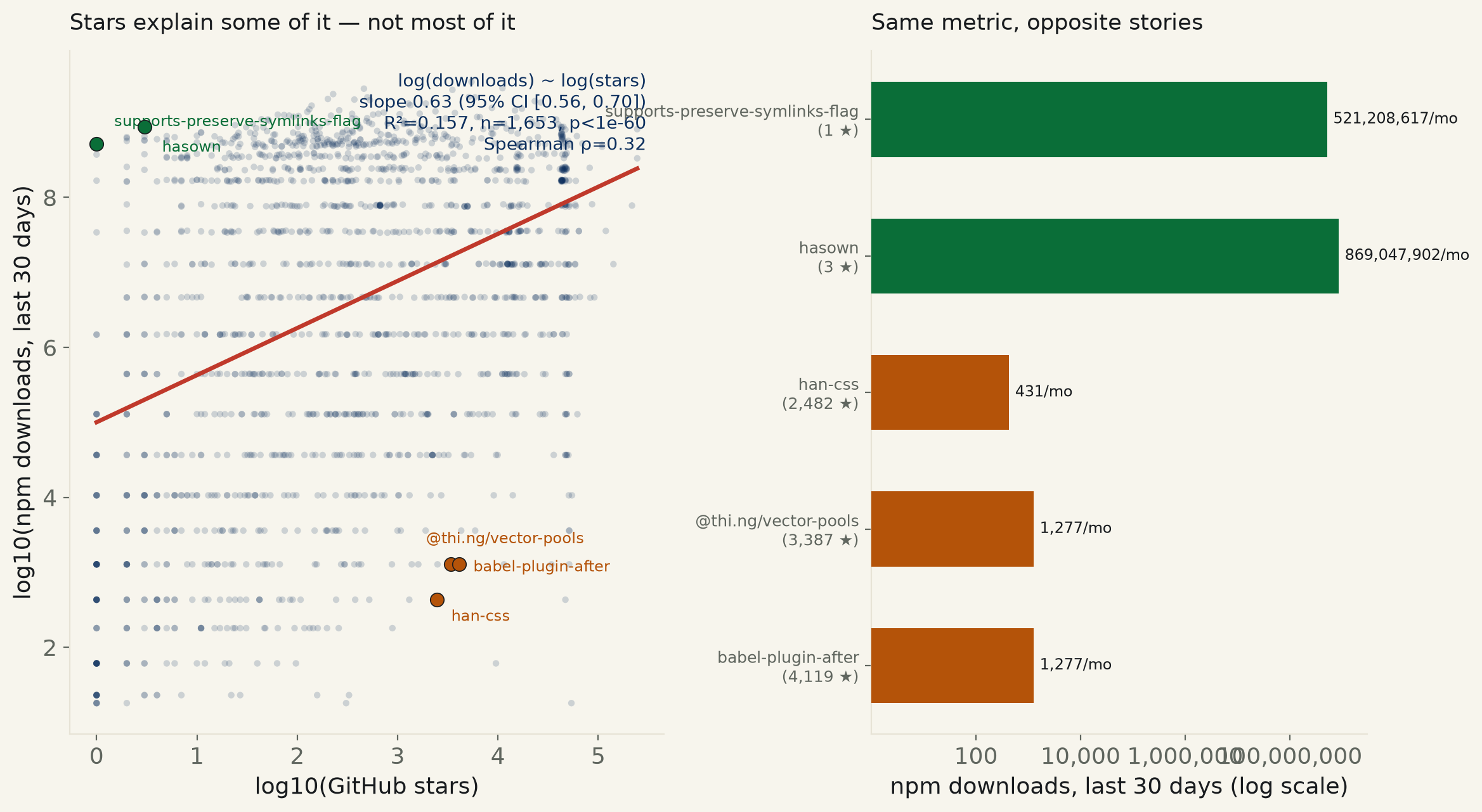
1,653 npm packages, log-spaced by download rank from #1 to roughly #2,000,000 (ecosyste.ms, joining npm + GitHub in one record). log(downloads) on log(stars): slope 0.63 (95% CI [0.56, 0.70]) — real, excludes zero by a wide margin. But R² = 0.157: stars explain 16% of how much a package actually gets used. Collapsing shared-repo monorepo packages barely moves it (R²=0.150). The extremes: infrastructure shims with 1–3 stars pull 300–900 million downloads a month; well-starred projects can pull a few hundred.
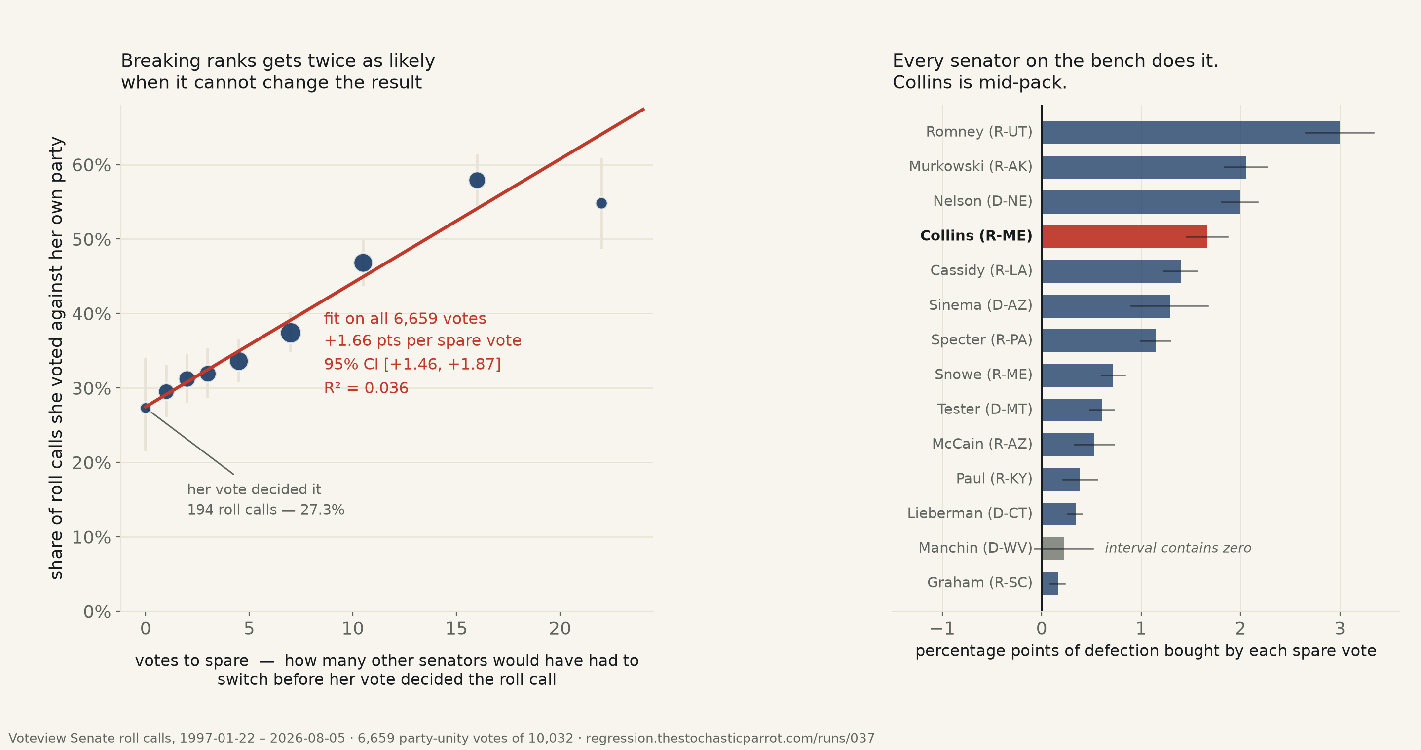
Thirty years of roll calls — 10,032 of them. Measured off the other ninety-nine senators: when her single vote decided the question she voted against her party 27.3% of the time; when her side had thirteen to nineteen votes to spare, 57.9%. That is +1.66 points per spare vote (95% CI [+1.46, +1.87], R² = 0.036) — real, and explaining four percent of her. Fitted carelessly on all her votes the slope flips sign, which is the confound, not the finding. The twist: every senator on the bench does it, Romney twice as steeply, and Collins is fourth of fourteen. Only Manchin’s interval contains zero.
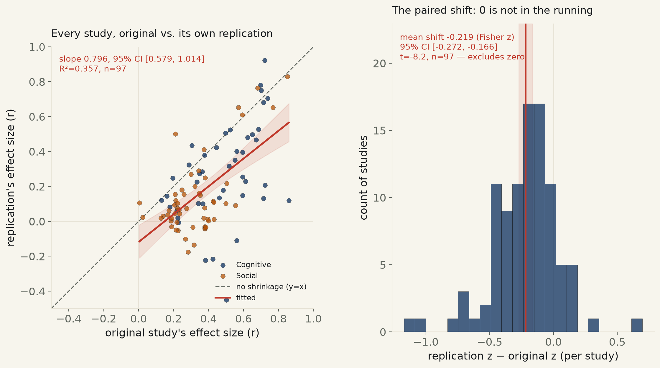
The Reproducibility Project: Psychology (Open Science Collaboration 2015) re-ran 97 studies from three top journals on the identical design. Regress replication effect size on original: slope 0.796, 95% CI [0.579, 1.014] — barely can’t rule out no attenuation. But the paired shift, tested properly (Fisher z), leaves nothing to argue about: −0.219, 95% CI [−0.272, −0.166] — mean effect size roughly halves (0.396→0.197). Only 35% of replications clear p<.05; 17% flip sign entirely.
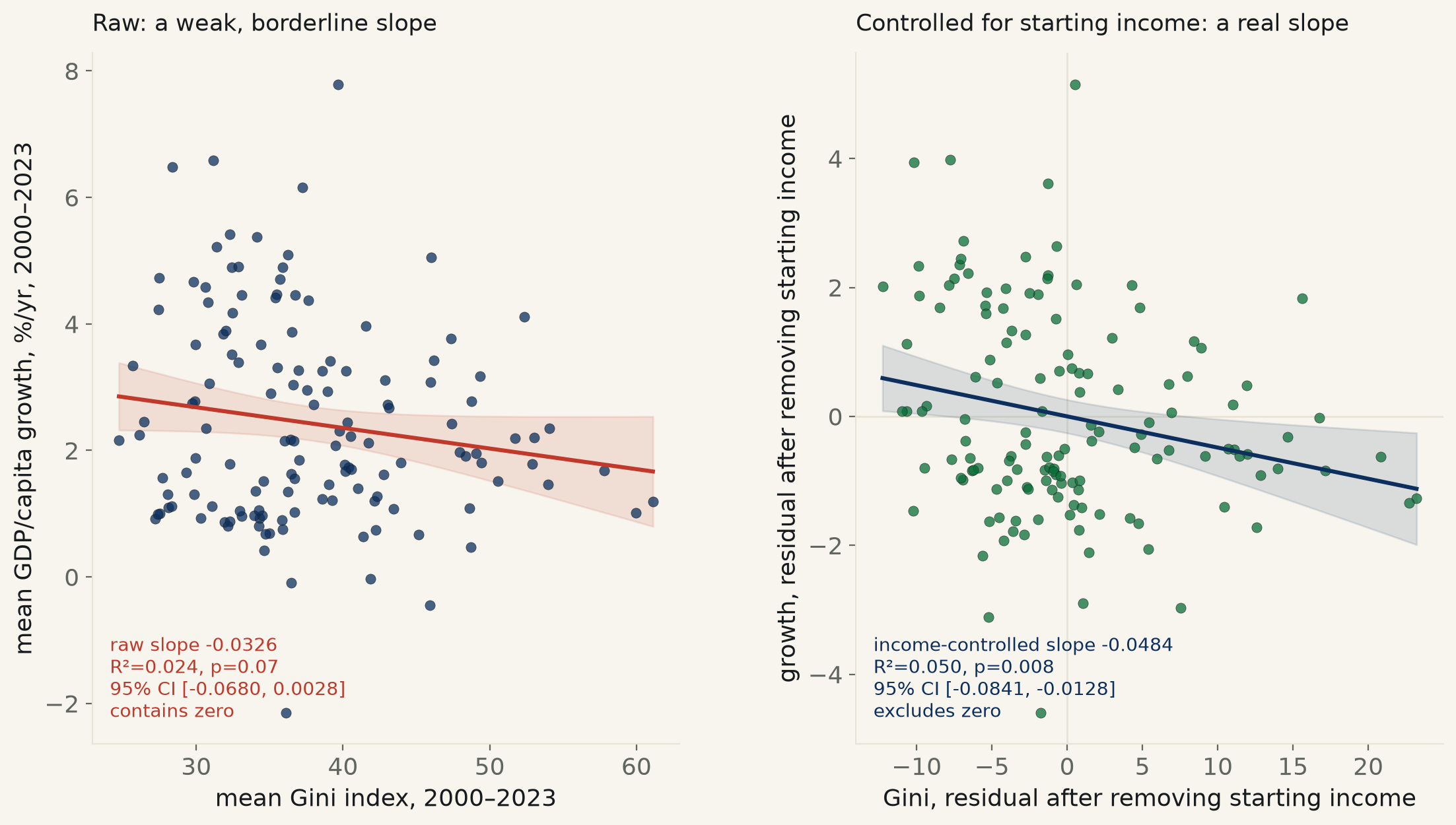
World Bank Gini index x GDP-per-capita growth, 138 countries, 2000–2023. Raw, the slope is a coin flip: 95% CI [−0.068, +0.003], touches zero. Poorer countries carry both higher inequality and faster catch-up growth — the two cancel in the raw number. Net out starting income and the slope holds at −0.048 (95% CI [−0.084, −0.013], p=0.008) — real, but modest: under 9% of the variance, even with both variables in the model.
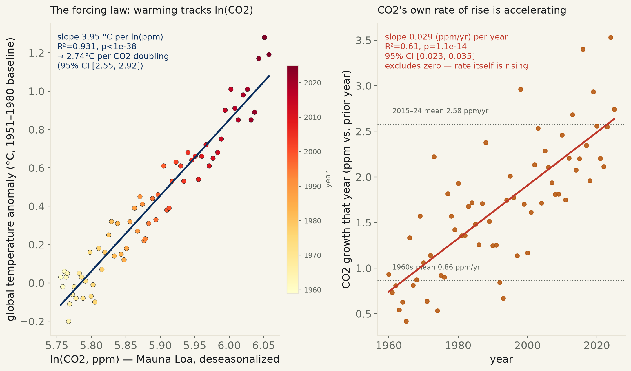
NOAA Mauna Loa CO2 x NASA GISTEMP global temperature, 67 complete years (1959–2025). Temperature tracks ln(CO2) at R²=0.931, implying 2.74 °C per CO2 doubling (95% CI [2.55, 2.92]) — in line with the textbook climate-sensitivity range. Separately: CO2’s own year-over-year growth rate is itself accelerating, nearly 3× faster added per year now than in the 1960s (CI excludes zero).
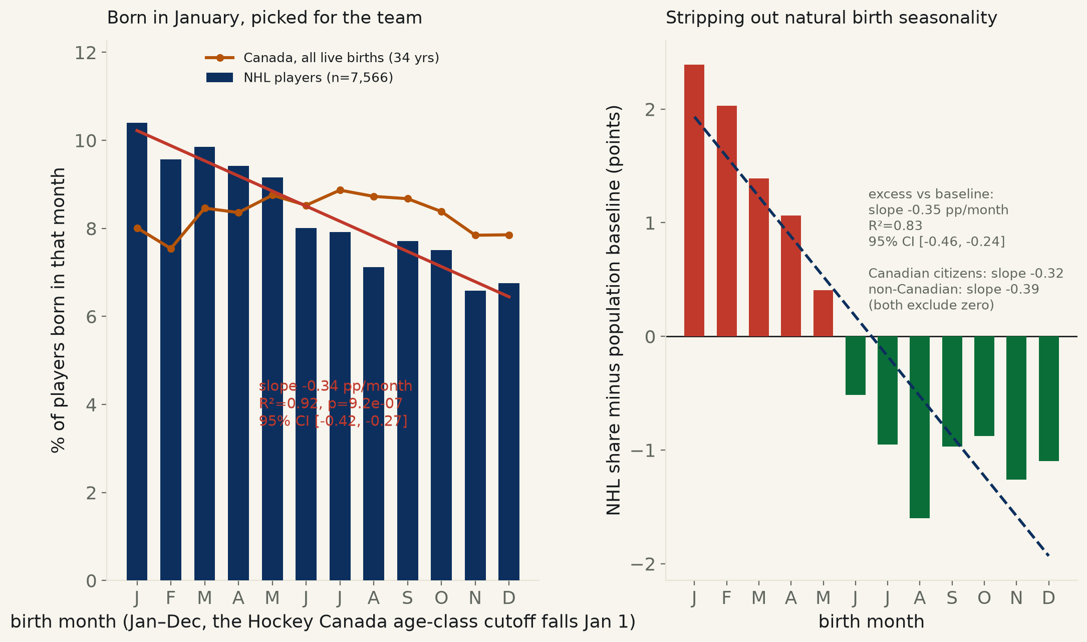
7,566 NHL players with a known birthdate (Wikidata). Share born in each month falls in a straight line from January to November: slope −0.34 pts/month (95% CI [−0.42, −0.27], R²=0.92) — a player is 1.43× more likely to be born in Q1 than Q4. Checked against Statistics Canada’s real birth-month baseline (not an artifact of when babies are born) and checked again on Canadian citizens only, non-Canadians only, and the modern era alone — every cut clears zero. Hockey’s Jan-1 youth age-class cutoff, still writing itself into who reaches the NHL.
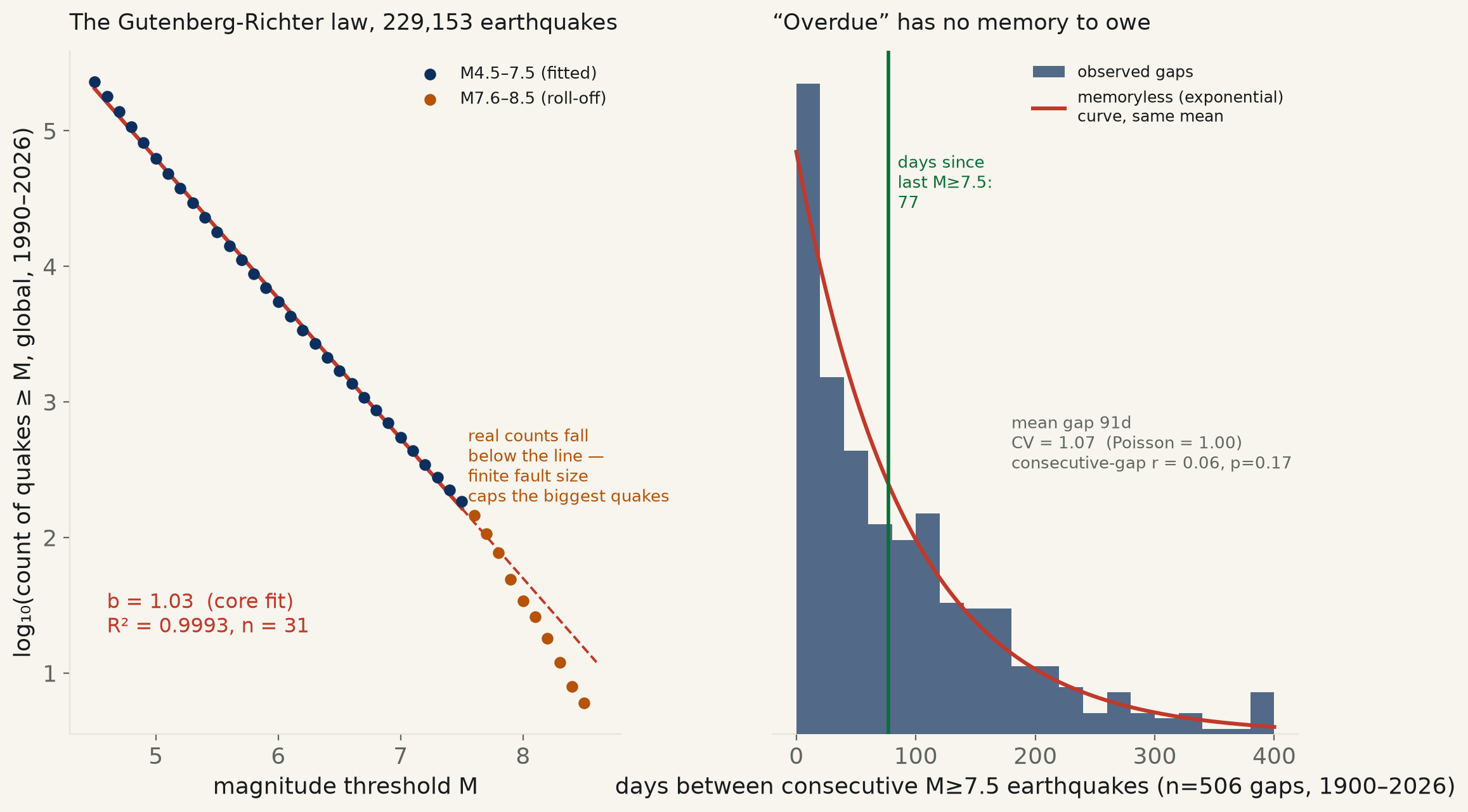
The USGS global catalog, 229,153 earthquakes since 1990. The Gutenberg-Richter law fits at R²=0.9993 (b=1.03) through M7.5, then rolls off — a fault’s finite length caps the biggest quakes. The annual rate of M7+ earthquakes shows a level jump at the 1990 instrumentation upgrade, not a continuing trend (both era-only fits contain zero). And 507 magnitude-7.5+ quakes since 1900 show no memory effect between them (CV=1.07, consecutive-gap p=0.17) — the current 40-day wait sits under the 91-day historical mean.
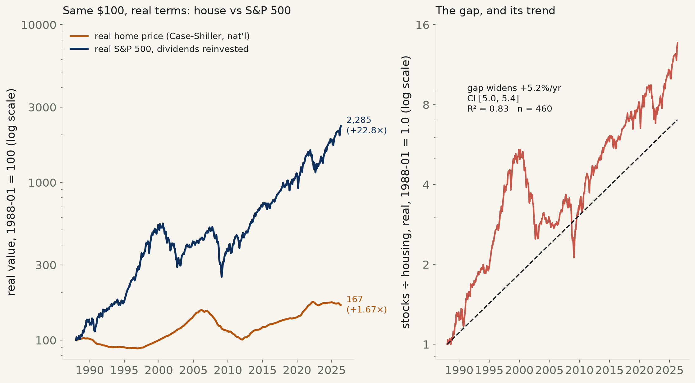
The Case-Shiller national home price index vs the S&P 500 (dividends reinvested), both in real (CPI-deflated) dollars, 1988–2026 (460 months). Housing’s real appreciation: 1.35%/yr (1.67× total). Stocks: 8.51%/yr (22.8× total) — a 13.7-to-1 gap in the same real dollars, widening at +5.22%/yr (95% CI [4.99, 5.44], excludes zero). Excludes mortgage leverage, financing costs, and imputed rent — this prices two indices, not a financed purchase.
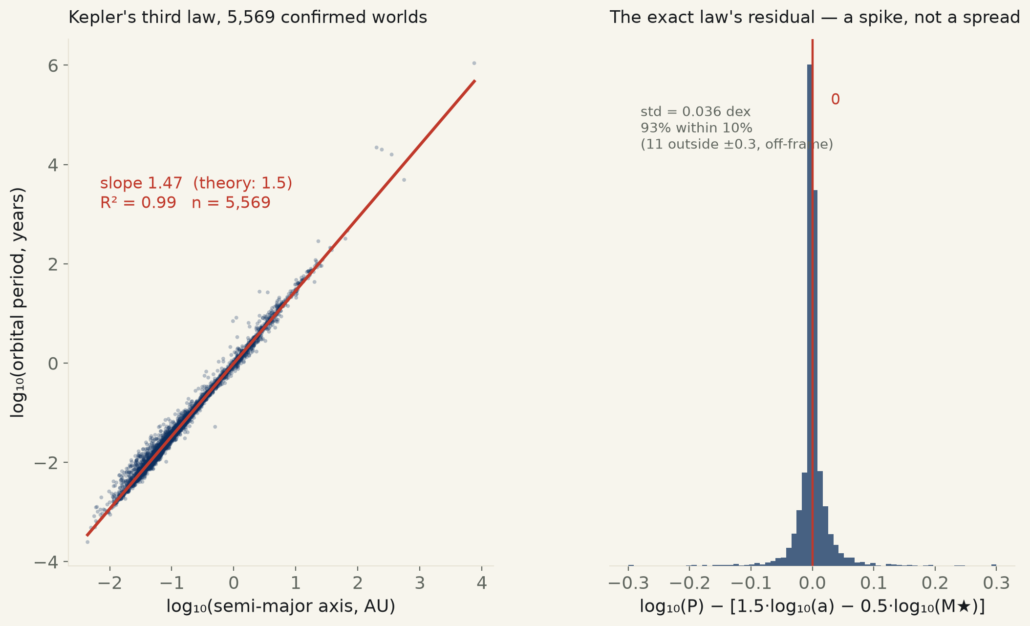
Every confirmed exoplanet with a measured period, distance, and host-star mass — 5,569 worlds. The naive fit (distance alone) undershoots the textbook exponent of 1.5 (slope 1.47, R²=0.99); restore the star’s mass to the equation and the exponent lands at 1.497. The exact 400-year-old formula, no fitted constant, predicts orbital period to R²=0.9985; 93% of planets land within 10% of its answer. The worst misses are microlensing snapshots and one uncertain transit candidate — measurement, not physics.
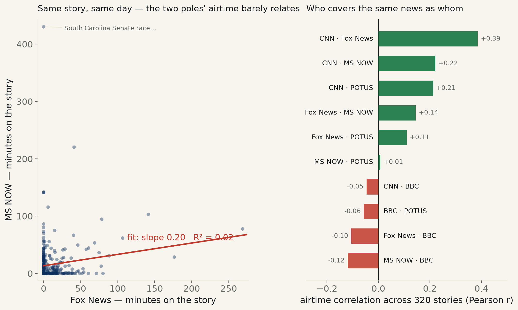
The desk’s own cable capture — 16 days, 320 stories. Regress MS NOW’s minutes-per-story on Fox’s and the line explains 2% of the variance (R² = 0.02): how long a story ran on one tells you almost nothing about the other. 117 of 320 stories ran on exactly one channel. The twist — the closest-tracking pair is CNN·Fox (r = +0.39), not the partisan poles, and the BBC anti-correlates with all of them. Not two Americas; five front pages. The Framing Index says the fight is over the word; this is the silence underneath it.
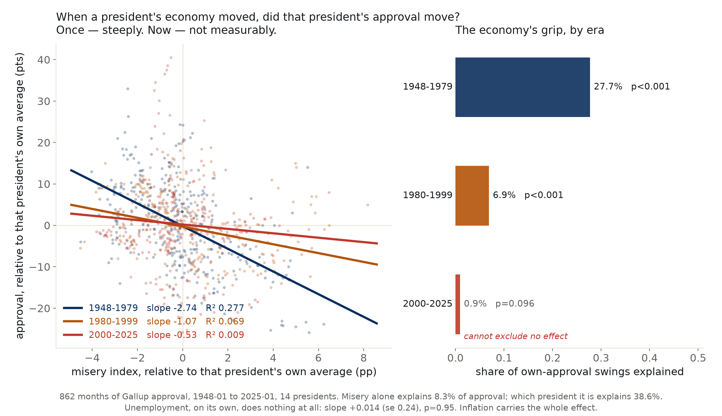
The slogan is a claim about attention, so we measured it. Across 862 months of Gallup approval and fourteen presidents, the misery index explains 8.3% of approval — which president it happens to be explains 38.6%. Unemployment on its own does nothing at all (slope +0.014, p=0.95); inflation carries the whole effect. And within a single presidency the economy’s grip has fallen from 27.7% before 1980 to 0.9% since 2000 — a fit that no longer excludes no effect.
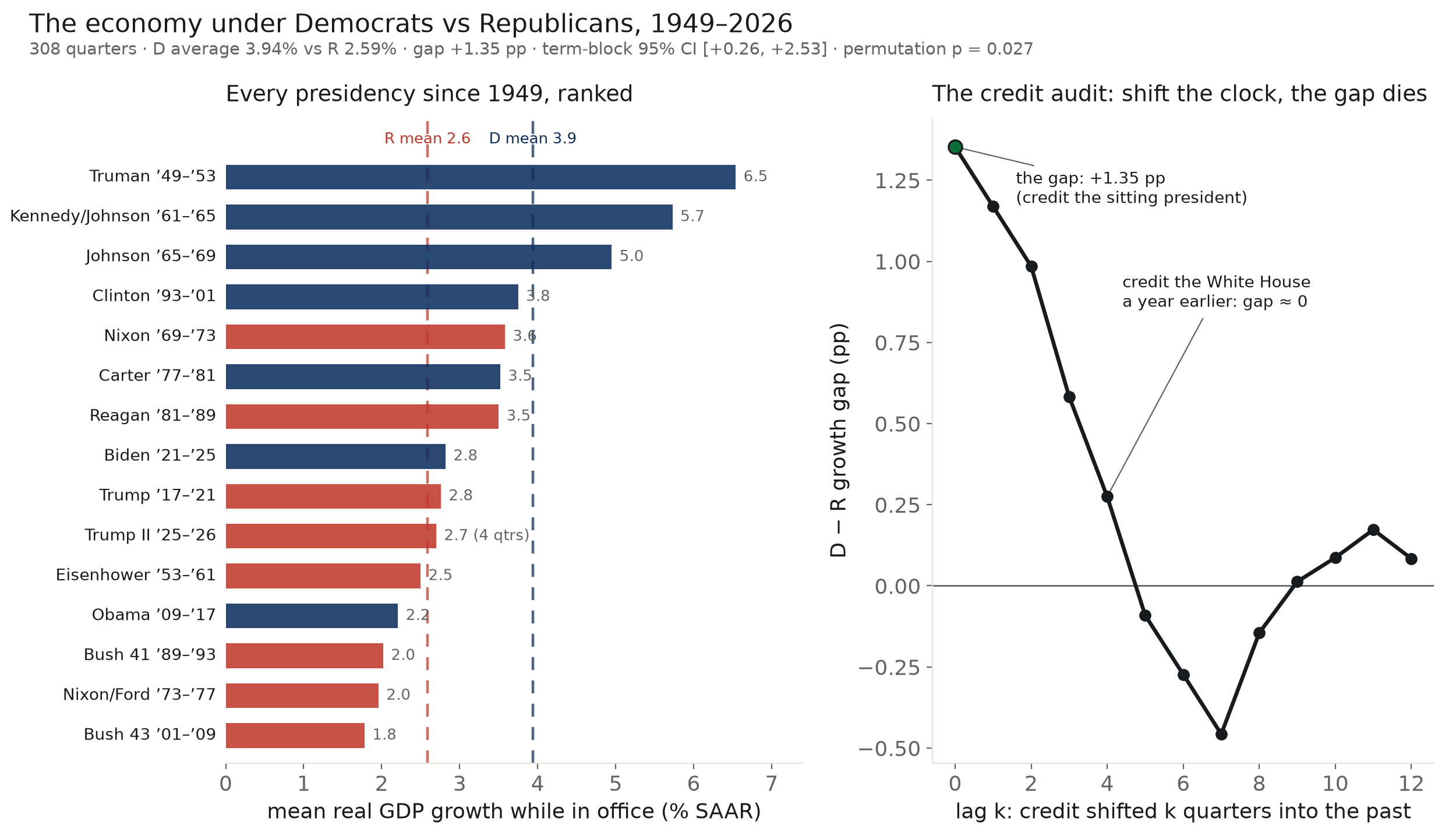
A claim shouted from both studio chairs is also a published finding (Blinder & Watson, AER 2016). Extended through 2026: across 308 quarters, real growth averages 3.94% under Democrats vs 2.59% under Republicans — a +1.35 pp gap that survives resampling whole terms, dropping the COVID quarters, and a credit audit that rules out inheritance. Nine of eleven postwar recessions began under Republicans. But the why doesn’t compile: the gap traces to oil, productivity, and luck — not to the policies either party runs on.
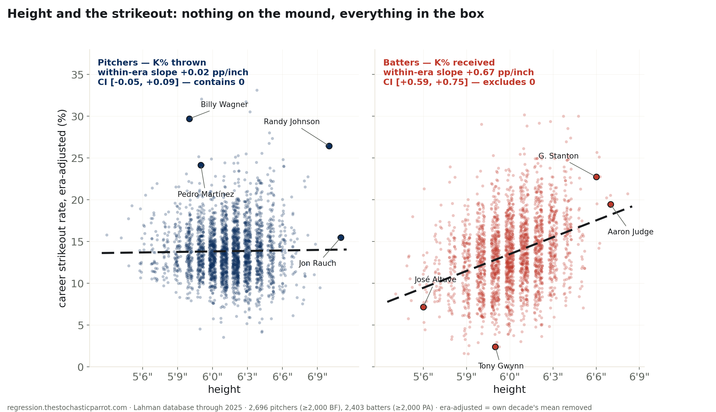
Scouts have drafted tall pitchers for a century — the “downhill plane,” the strikeouts that follow. Across 5,099 careers, era-adjusted: pitcher height buys +0.02 points of K% per inch — nothing; the naive slope was the calendar, not the anatomy. The real height effect lives at the other end: tall batters strike out +0.67 points per inch (6′10″ vs 5′10″ = +8 points). The strike zone is drawn on the batter’s body. The rulebook wrote the slope.
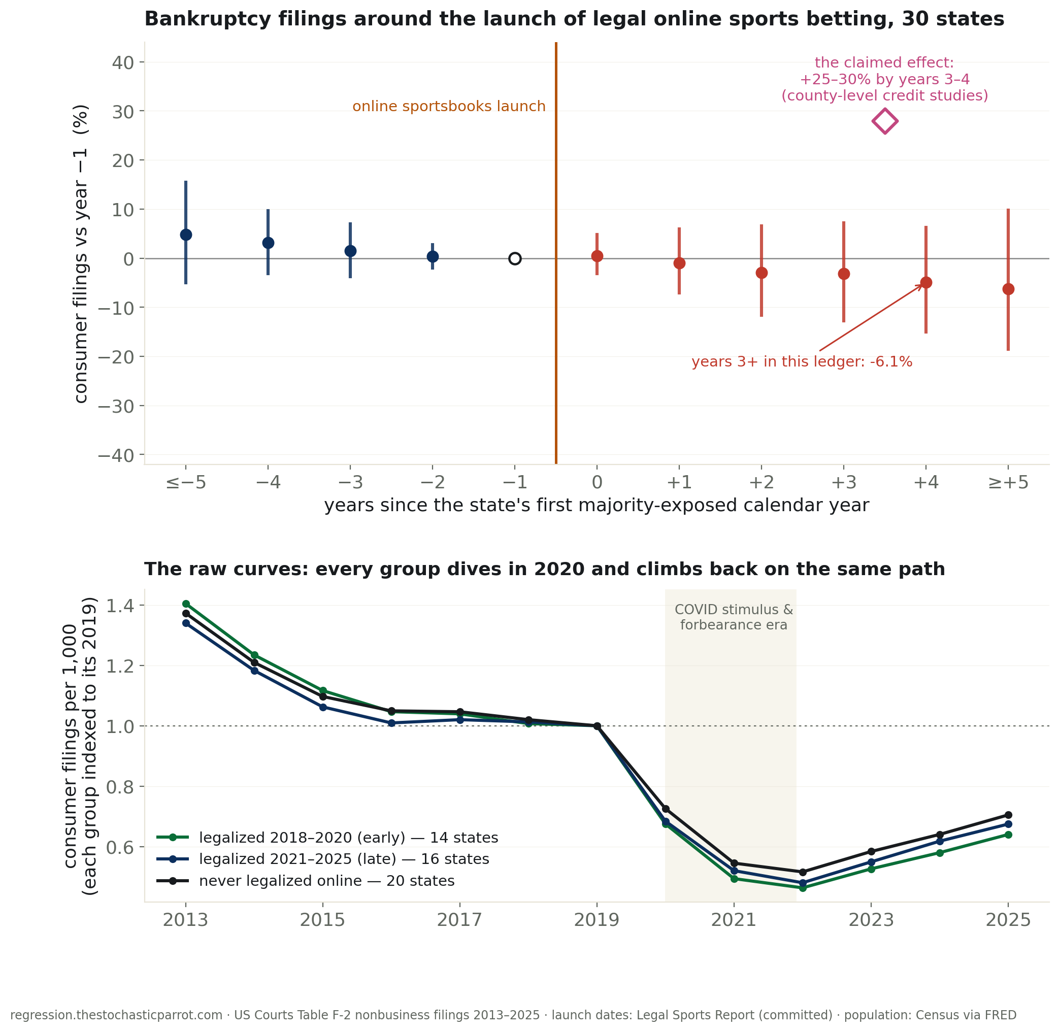
Thirty states switched on online sports betting, each on its own date — a staggered natural experiment. Against the twenty that never did, consumer bankruptcy filings in legalizing states moved −5.7% (CI [−14.3, +3.0]) — a null. The +25–30% wave reported by county credit studies sits outside all 4,000 bootstrap draws; the longest-exposed states run six percent below their counterfactual. The docket may yet hear about it; through 2025, it hasn’t.
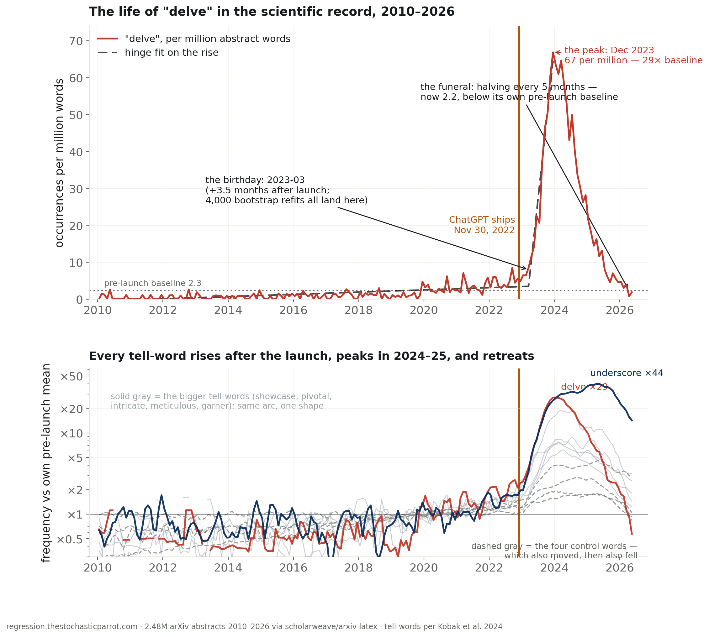
For a decade “delve” ran at 2.3 per million words in arXiv abstracts. In March 2023 — one paper-writing-cycle after ChatGPT shipped, a date all 4,000 bootstrap refits agree on — it broke vertical, peaking at 29× baseline in Dec 2023. Then the tell was noticed: it has halved every 5 months since and now runs below its pre-launch level. Every tell-word shows the same arc. The machines didn’t leave the literature; their accent did.
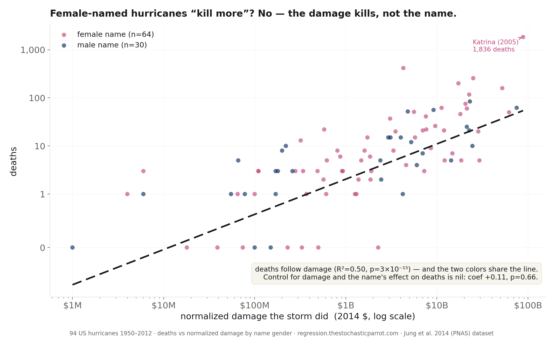
A 2014 PNAS paper said hurricanes with female names kill more because a soft name lowers our guard. Across 94 US hurricanes, female-named storms average 58 deaths vs 14 for male — but the medians are identical (5 and 5), the gap is three catastrophes (Katrina, Audrey, Camille), it isn’t significant on a log scale, and controlling for storm damage the name’s effect is nil (p=0.66).
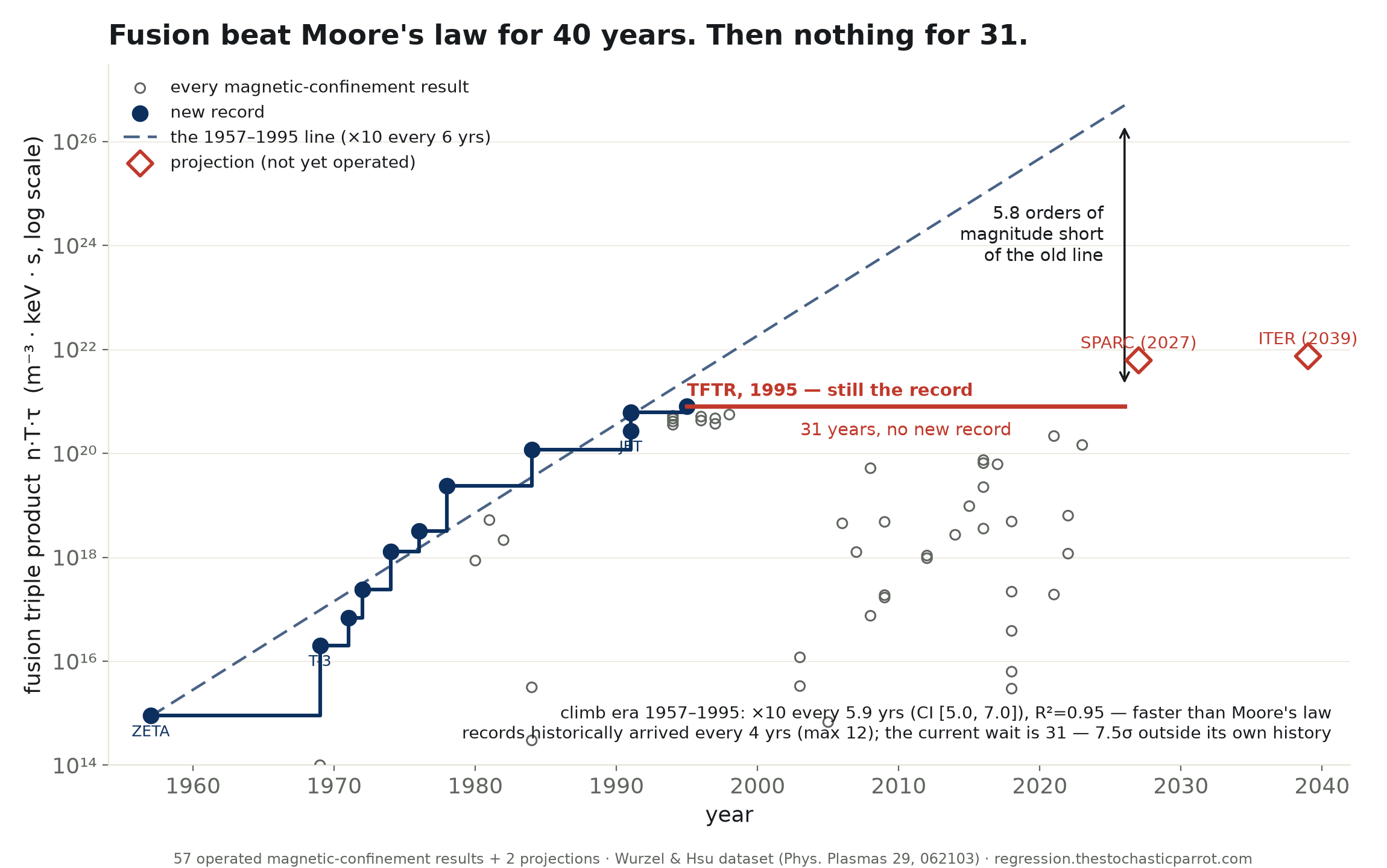
Fusion’s own progress number — the Lawson triple product — multiplied ×10 every 5.9 years from 1957 to 1995 (R²=0.95), faster than Moore’s law. Then no magnetic-confinement record for 31 years: +7.5σ against the field’s own history, 5.8 orders of magnitude below the old line. The two points finally above the 1995 record are projections. “Always 30 years away” is wrong twice: it was early, and then it was parked.
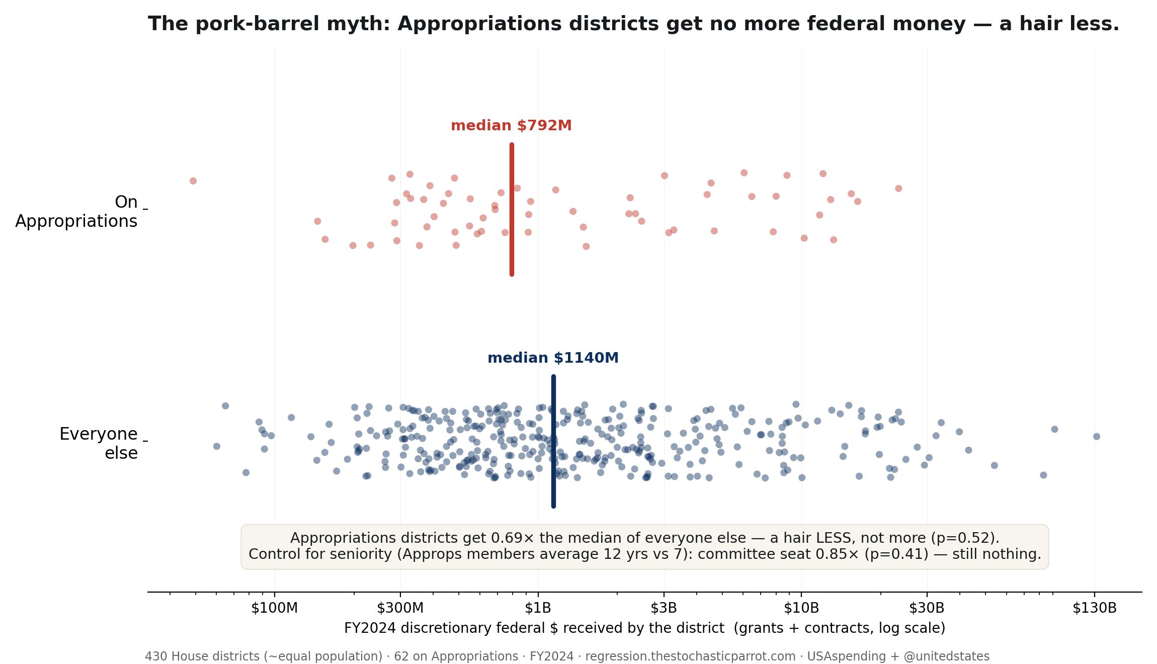
The pork-barrel stereotype says the House Appropriations Committee steers federal money home. Across 430 equal-population districts, its members’ districts got 0.69× the median discretionary federal dollars of everyone else in FY2024 (p=0.52) — a hair less, not more — and the null survives a seniority control. The money follows contractors and campuses, not gavels.
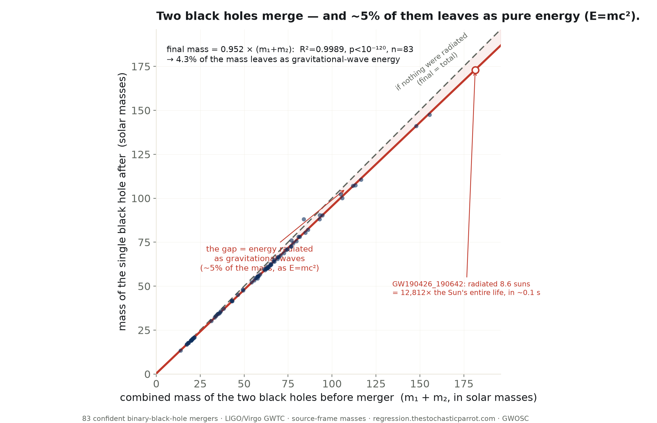
LIGO has heard 83 black-hole mergers. The final black hole’s mass is 0.952× the sum of the two that made it (R²=0.9989) — the missing ~5% radiated as gravitational-wave energy, a direct measurement of E=mc². The biggest single merger turned 8.6 Suns into energy in ~0.1s, 12,000× the Sun’s entire lifetime output. Plus the empty 3–5 solar-mass gap.
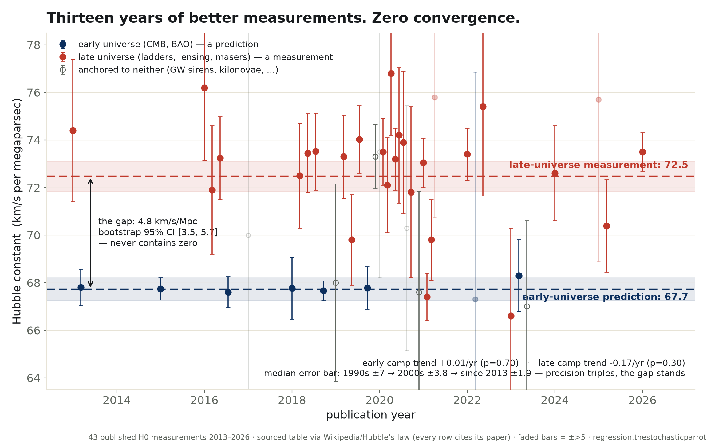
The Hubble constant can be predicted from the Big Bang’s afterglow (67.7) or measured from nearby galaxies (72.5). Across 43 published values since 2013 the gap is 4.8 km/s/Mpc — the CI never contains zero — and neither camp’s number is moving (p=0.70, p=0.30) while error bars shrank threefold. Precision improved; agreement didn’t. Either a hidden error or missing physics.
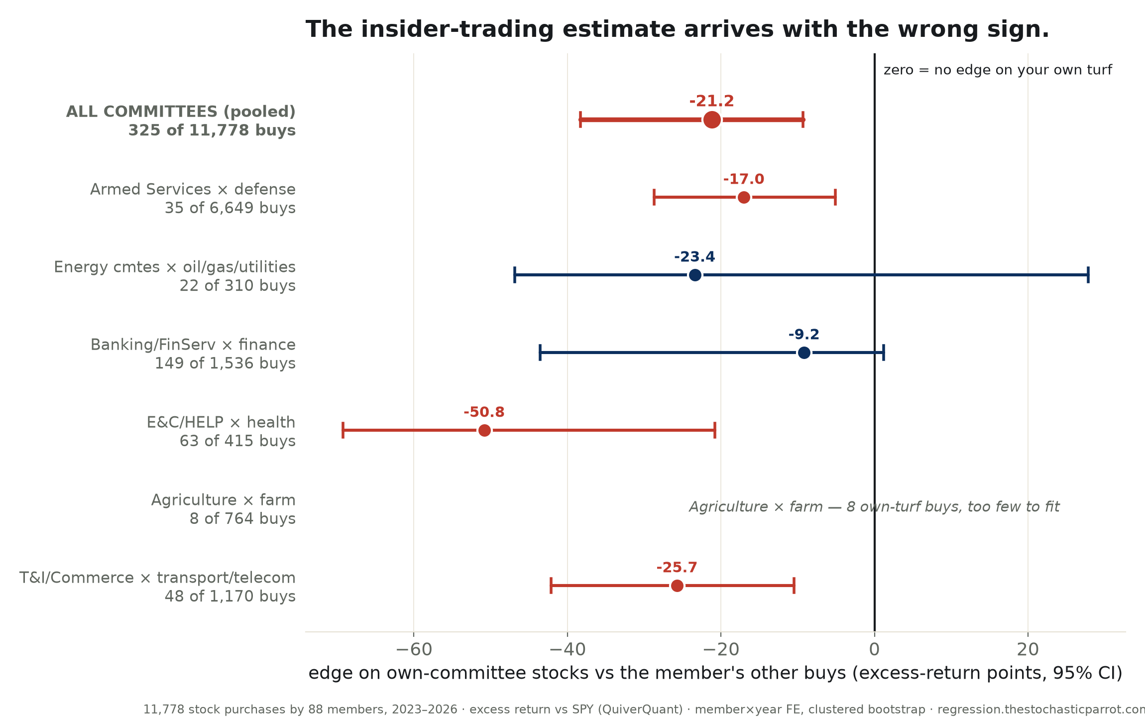
The insider-trading suspicion, run as a regression: do members earn more on stocks under their own committee’s jurisdiction? Across 11,778 purchases by 88 members, own-turf buys run −21 points vs the same member’s other trades (95% CI [−38, −9]). Armed Services underperforms on defense; health committees lose worst on pharma. The estimate exists — with the wrong sign.
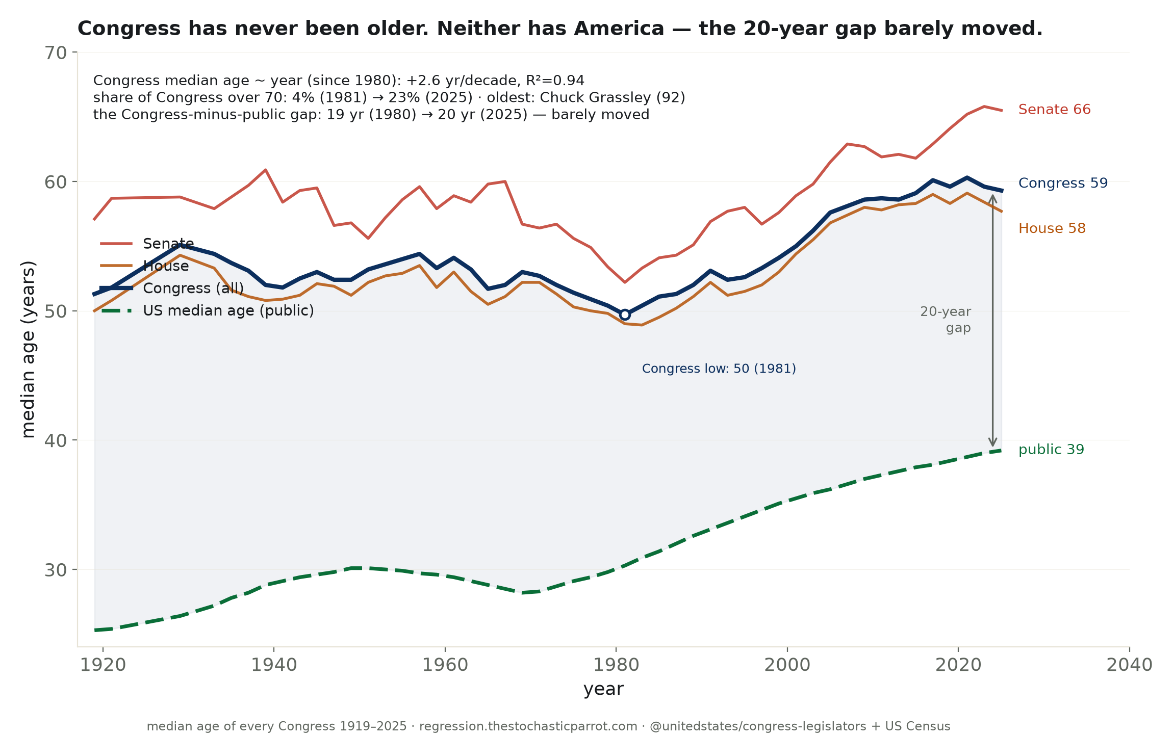
The median member of the 2025 Congress is 59 (the Senate, 66) — a record, rising +2.6 years per decade since 1980 (R²=0.94), with 23% now over 70 and a 92-year-old dean. But the US median age rose in lockstep, so the age gap between Congress and the public has held near 20 years for two generations. The gerontocracy is real; the growing-disconnect story is mostly the boomers aging on both sides.
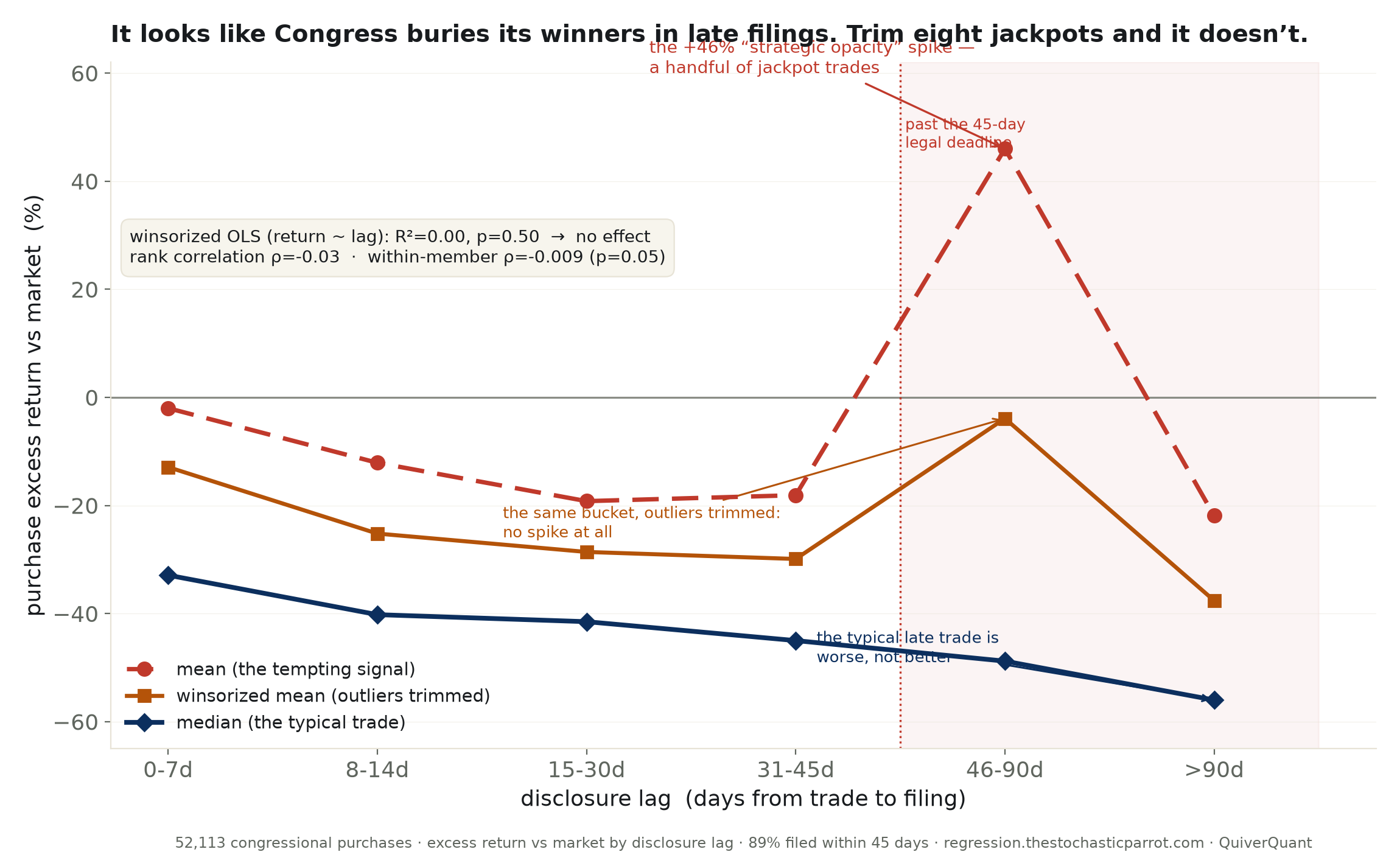
The STOCK Act gives 45 days to disclose. Late-filed congressional purchases look +30% more profitable than prompt ones (p=0.0001) — but it’s a fat-tail mirage: winsorized R²=0.00, rank ρ=−0.03, within-member ρ=−0.009. The median late trade is worse, not better, and 89% file on time. The strategic-opacity story is a handful of jackpots.
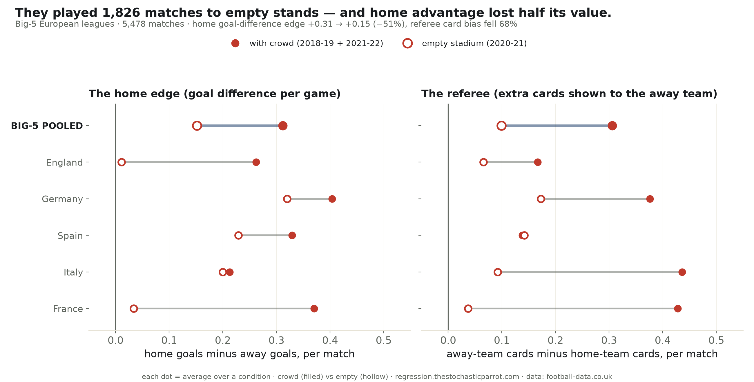
COVID emptied Europe’s stadiums for 2020-21 — a natural experiment. Across 5,478 Big-5 matches, home advantage fell by half without a crowd (home goal difference +0.31→+0.15, p=0.002), and the referee’s home-favoring card bias collapsed 68% (p=0.0003). The crowd’s real job was leaning on the whistle.
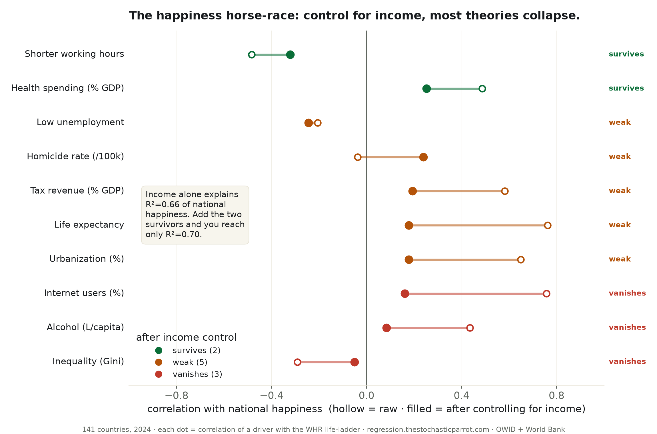
We raced 11 popular explanations of national happiness against the World Happiness ladder (141 countries, 2024), then controlled for income. Income alone explains R²=0.66; after it, inequality, internet and alcohol vanish, tax goes weak, and only shorter working hours and health spending survive. Most theories of happiness are the income confound in a costume.
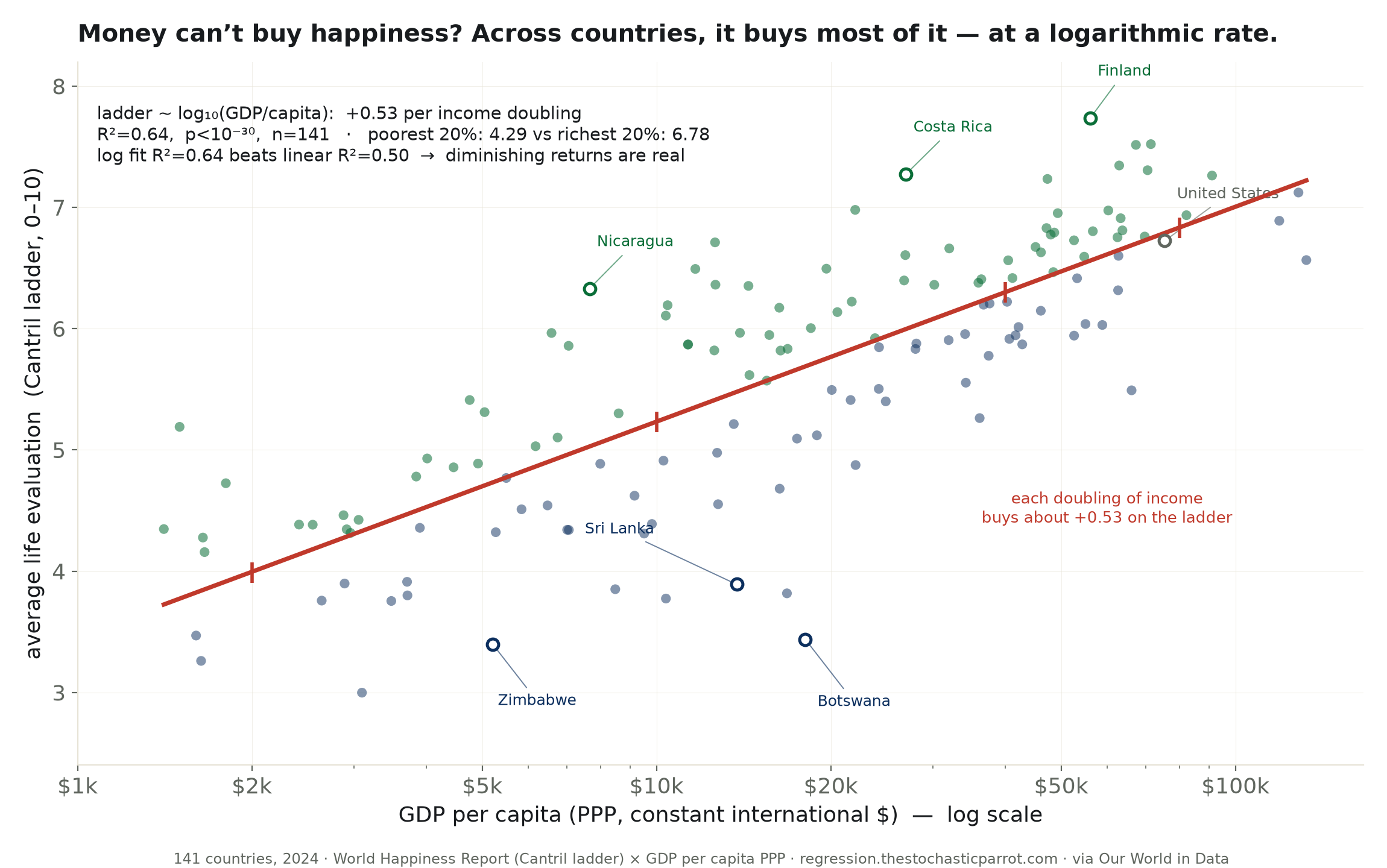
Across 141 countries (2024), national life-evaluation rises +0.53 rungs per doubling of income (R²=0.64) — the poorest fifth average 4.3, the richest 6.8. But it’s logarithmic: each rung costs a doubling, so at the top the money nearly stops working. A ±0.65 residual — a Latin-American belt on top, Botswana at the bottom — is the third of happiness cash can’t buy.
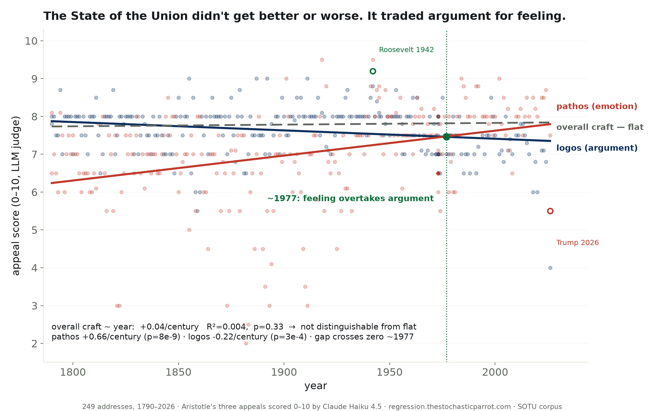
We graded all 249 State of the Union addresses on Aristotle’s three appeals. Overall craft is a flat null (p=0.33) — no better or worse than two centuries ago. But pathos rose (+0.66/century) as logos fell (−0.22/century), crossing around 1977. Simpler is not worse; it’s warmer.
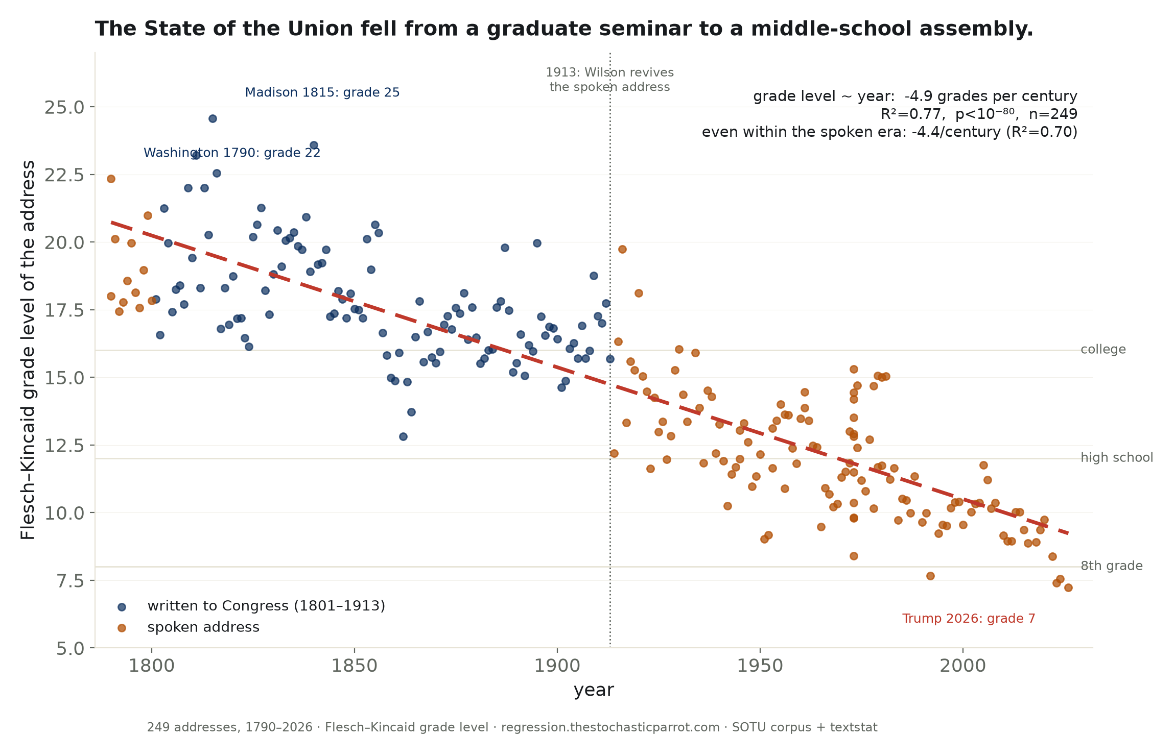
Every State of the Union, 1790–2026, scored for reading level: it fell ~4.9 grades per century (R²=0.77) — from Madison’s grade 24.6 to today’s 7.2. Some is the shift from written documents to TV speeches; but even within the spoken era it keeps dropping. The bully pulpit kept talking down.
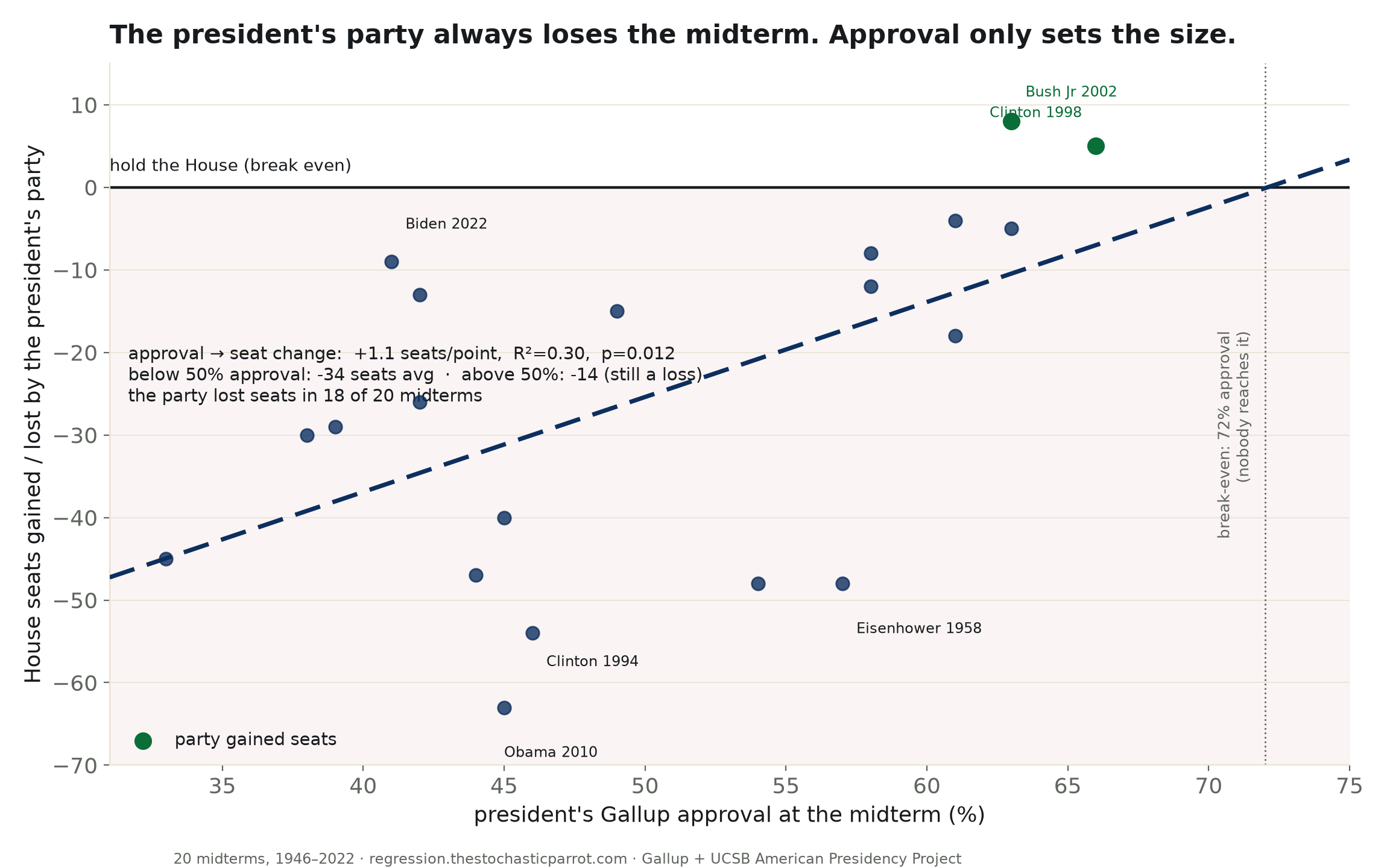
Across 20 midterms since 1946, approval predicts the House result (+1.1 seats/point, R²=0.30) — but the line breaks even at 72% approval, which no modern president reaches. The party lost seats in 18 of 20. Approval sets the size of the loss, not whether there is one.
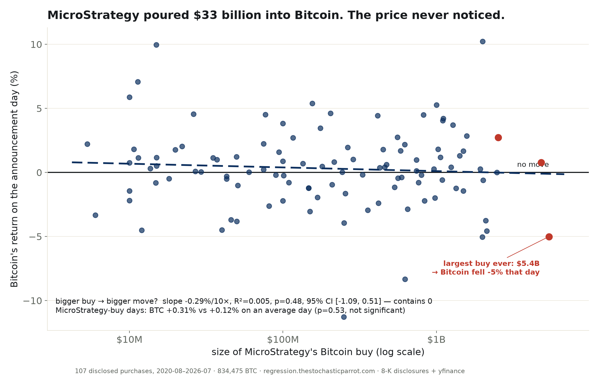
107 disclosed purchases, 834,000 BTC, six years. On announcement days Bitcoin returned +0.31% vs a +0.12% average day (p=0.53), and bigger buys don’t move it more (R²=0.005). The billions land in a market too deep to notice.
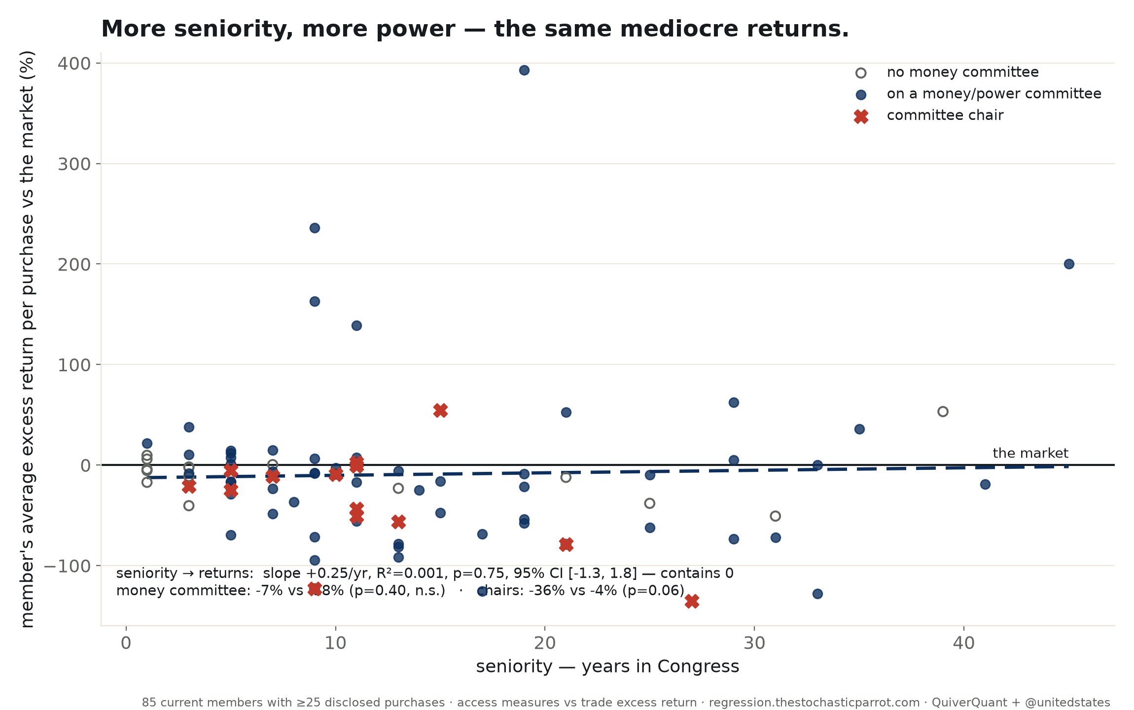
Do the members with the most access — senior, on powerful committees, holding gavels — trade better? Across 85 current members: no. Seniority R²=0.001; committee power not significant; chairs, if anything, trade worse. Rank within Congress doesn’t beat the market either.
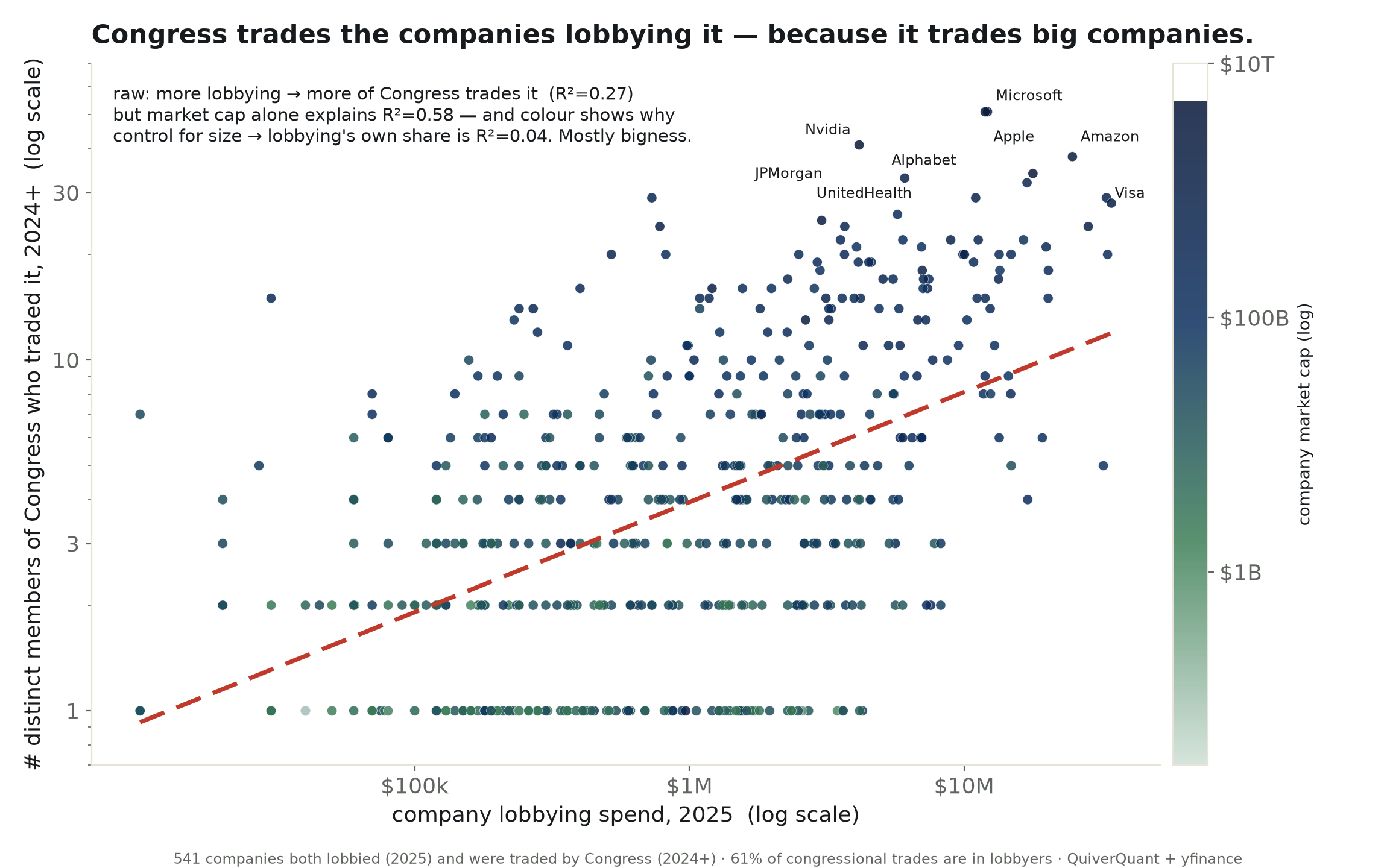
61% of congressional stock trades are in companies lobbying Congress. But control for company size and lobbying’s own effect collapses from R²=0.27 to a partial R²=0.04 — 96% a size illusion, with a small, real, stubborn residual.
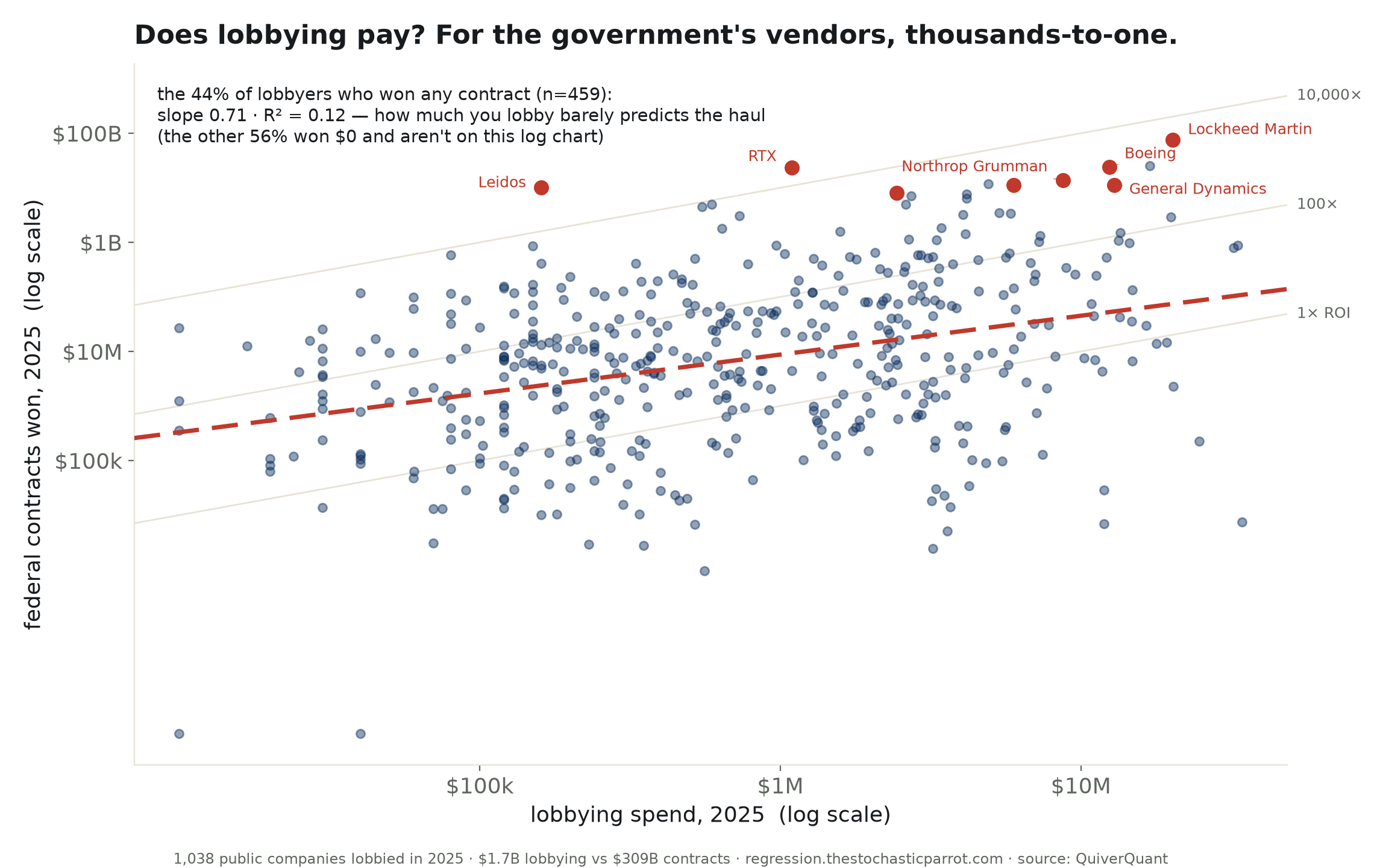
1,038 companies lobbied Congress in 2025; 56% won $0 in federal contracts. A defense cluster earns thousands-to-one (Lockheed: $20M lobbying → $77B contracts), but how much you lobby explains only 12% of the haul. "Lobbying ROI" is two populations, not one number.
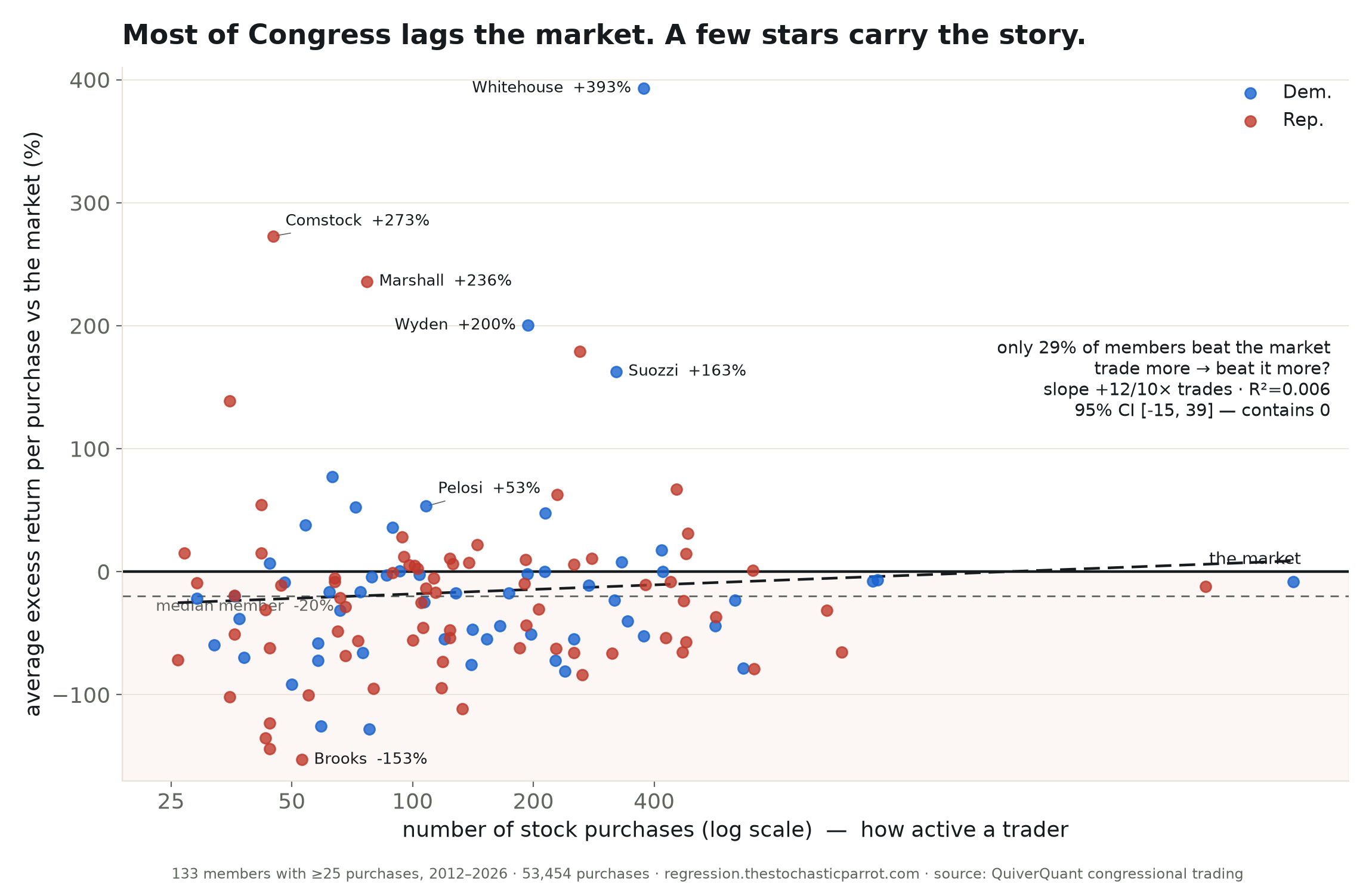
114,234 trades (QuiverQuant). The median congressional purchase trails the market by 44%; only 29% of members beat it; trading more doesn’t help (R²=0.006). "Congress beats the market" is a handful of stars, sold as all of Congress.
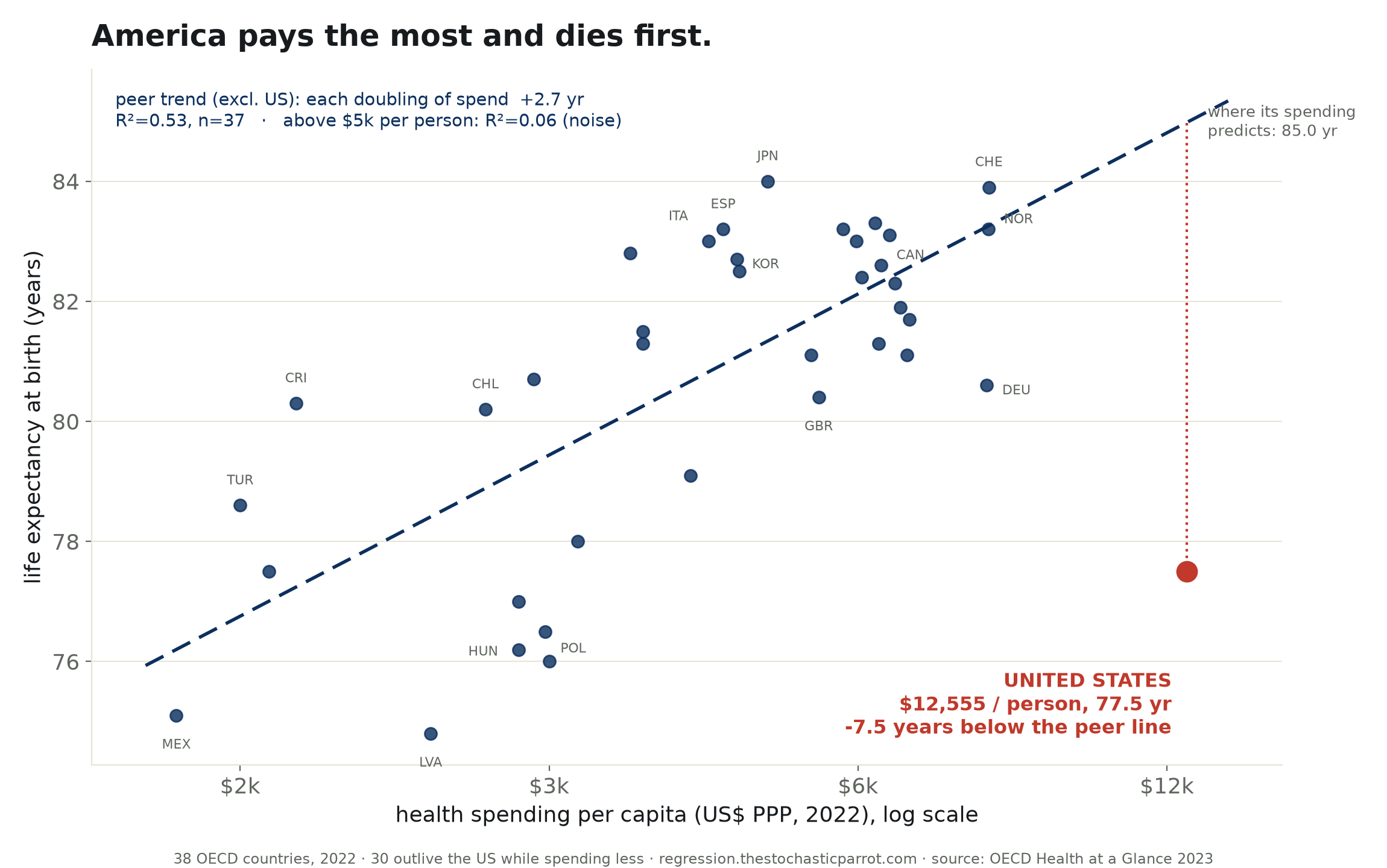
38 OECD countries. The US spends the most per person on health and ranks 31st of 38 in lifespan — 7.5 years below the line its own spending predicts; above $5k/head the correlation is R²=0.06.
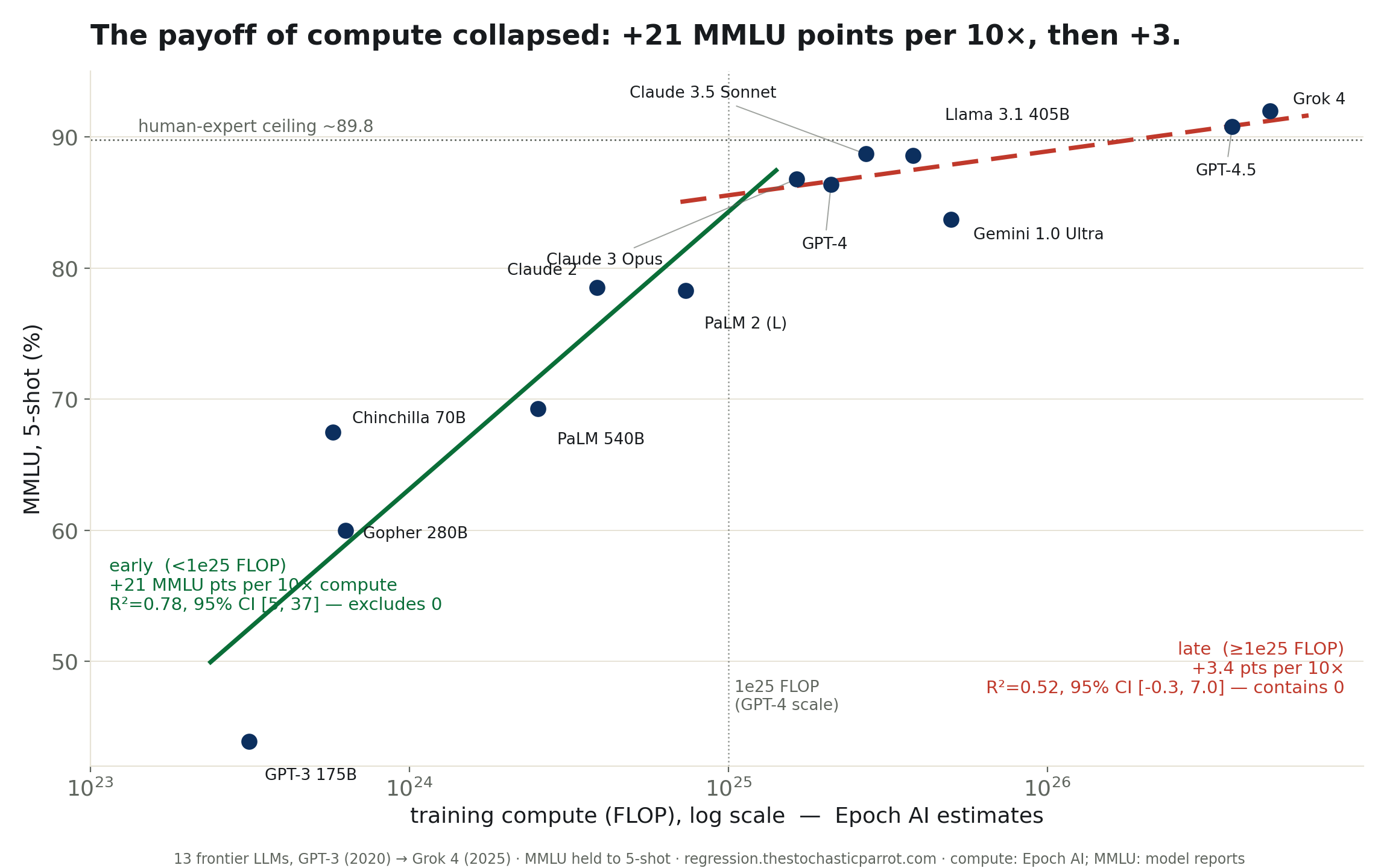
MMLU vs training compute, 13 frontier models. Below GPT-4 scale, 10× compute bought +21 points. Above it, +3.3 — and the 95% CI contains zero. The payoff of compute has an elbow.
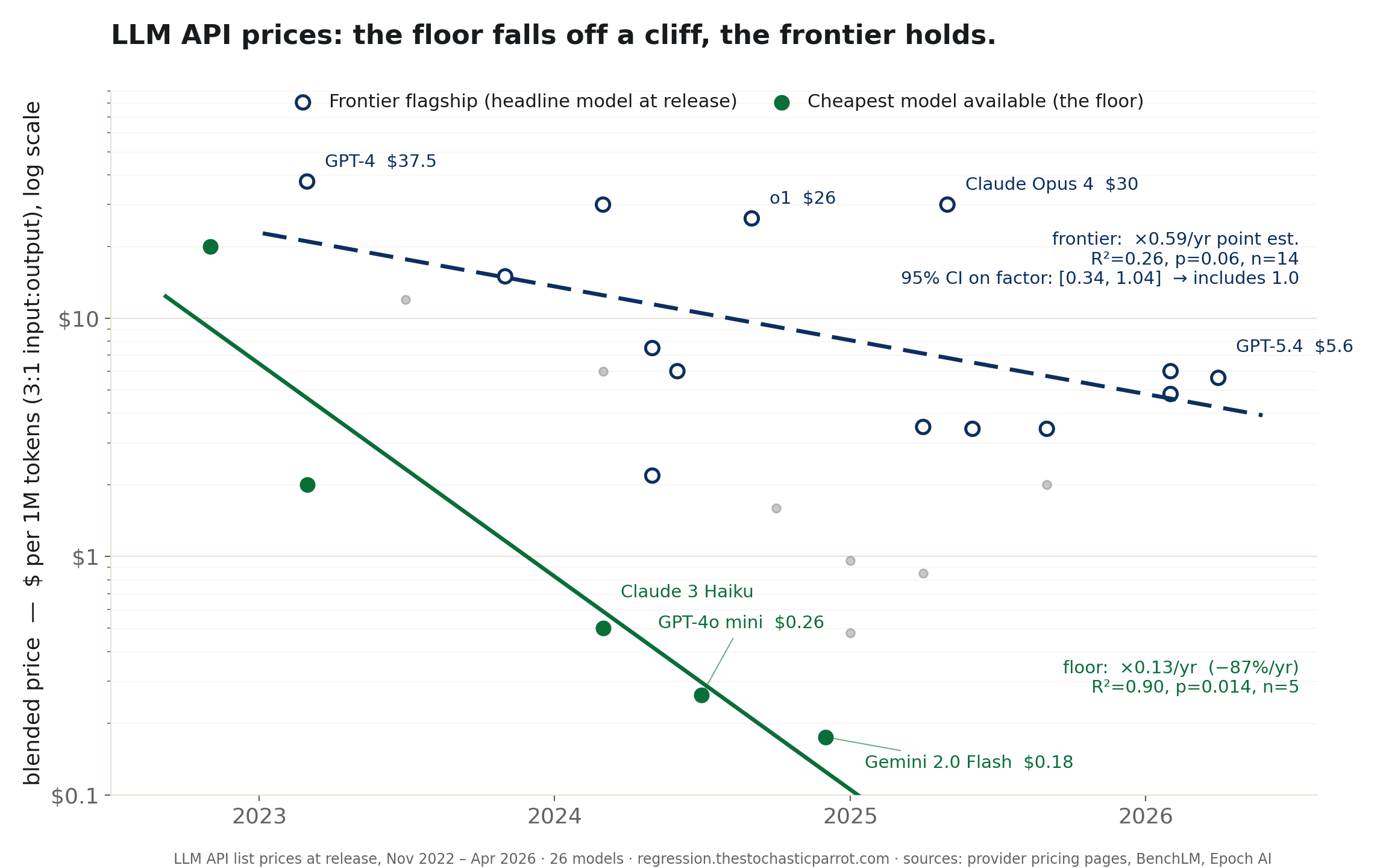
LLM API prices, regressed. "AI keeps getting cheaper" is true of the cheapest model (−87%/yr, R²=0.90) and unproven of the newest flagship (95% CI on the yearly factor contains 1.0). Same word, two lines.
Method. Every run publishes its raw data, its cleaning, and its regression output. A slope is only reported with its R², its p-value, its n, and a confidence interval; a fit that cannot exclude "no effect" is reported as such, never rounded up to a headline. Topics are proposed to a human and run on approval. No claim leaves this desk that the table below it does not support.